` 1

https://www.youtube.com/watch?v=aNrqaOAt5P4&list=PLQY2H8rRoyvzuJw20FG82Lgm2SZjTdIXU&index=2


- 이번 동영상은 모델이 글을 읽는 학습 과정을 케라스를 통해 보여줍니다.

- 사람이 유치원을 다닐 때 글을 배우는 과정이 신경망이 글을 배우는 과정과 동일하다면서 영상을 시작합니다.

- NLP는 계속해서 진화하는 중이고, 사람 수준을 뛰어넘었습니다.


데이터 준비하기

- 신경망이 학습하기 위해선 데이터가 필요합니다. corpus와 같은 데이터말이죠.
먼저, 데이터를 확인해보겠습니다.
(데이터는 영상으로 대체합니다.)

lines = tf.data.TextLineDataset('./CBTest/data/cbt_train.txt')

for line in lines.take(3):
  print(line)

이 데이터를 그대로 사용하면 위험합니다. 데이터를 클린하게 만들어 줄 필요가 있습니다.

lines = lines.filter(
    lambda x: not tf.strings.regex_full_match(x, "_BOOK_TITLE_.*")
)

punctuation = r'[!"#$%&()\*\+,-\./:;<=>?@\[\\\]^_'{|}~\']'
lines = lines.map(lambda x: tf.strings.regex_replace(x, punctuation, ' '))

위의 결과와 비교해보세요. 클린해진 것을 한눈에 알 수 있습니다.

이제 모델에 데이터를 입력하기 위해 window 형태로 만들어야 합니다. 모든 문장의 길이는 같기 때문에 단순히 split만 해주면 되겠군요.

words = lines.map(tf.strings.split)
wordsets = words.unbatch().batch(11)

for row in wordsets.take(3):
  print(row)

모델이 정답은 알아야겠죠? 데이터의 마지막 단어를 레이블로 만들고 싶습니다.

def get_example_label(row):
  example = tf.strings.reduce_join(row[:-1], separator = ' ')
  example = tf.expand_dims(example, axis = 0)
  label = row[-1:]
  return example, label

data = wordsets.map(get_example_label)
data = data.shuffle(1000)

결과는 다음과 같습니다. 한 개의 긴 문장(학습용 데이터), 한 개의 레이블로 이루어져 있네요.

하지만 신경망 모델이 직접 언어를 배울 수는 없습니다. 오로지 숫자를 배울뿐이죠.
그래서 위와 같은 데이터를 다시 숫자로 변환해야 합니다.

vocab_size = 5000 # Maximum vocab size
vectorize_layer = tf.keras.layers.experimental.preprocessing.TextVectorization(max_tokens=vocab_size,
                                                                               output_sequence_length = 10)

이와 같은 전처리 레이어는 다양하게 keras에서 제공하고 있으며, tf.data.Datasets와 활용하면 매우 효과적입니다. 다음 그림에서 전처리 레이어가 얼마나 다양하게 존재하는지 알 수 있습니다.


모델 준비하기

이제 모델을 구성하면 됩니다.(seq2seq 모델)
케라스와 TensorFlow AddOnes를 활용하면 쉽게 구성할 수 있습니다. seq2seq 모델은 상당히 복잡한데, Encoder는 keras layer를 통해 쉽게 구성할 수 있고,  Decoder는 AddOnes를 활용하여 한번에 구성할 수 있는 것을 영상에서 보여줍니다.

TF 2.x에서는 학습 과정을 클린하고 모듈화된 과정을 제공하기 위해 노력한다고 합니다.
train_step을 직접 만들고, Gradient_Tape()를 활용하여 모델을 업데이트시키죠.

학습 단계를 정의했다면, 기존의 케라스와 동일하게 compile() 함수를 활용해서 과정을 설정합니다.
그래서 위의 train_step을 직접 정의해야 되냐고요?
model.fit() 함수를 사용하면 위의 과정이 전부 포함되어 있습니다.

model = MyModel()
model.compile(...)
model.fit(...)

케라스를 사용해서 우리는 만족할 수준의 모델 성능을 쉽게 얻을 수 있었습니다.
하지만 아직 하이퍼파라미터 튜닝을 진행해보지 않았군요.


하이퍼파라미터 튜닝하기

KerasTuner를 활용한다면 매우 쉽습니다!
코드에서 hp(hyperparameter 객체) 인자를 사용해 튜닝을 준비하고 있습니다.

import kerastuner as kt

def build_model(hp):
  model = EncoderDecoder(
    			rnn_units = hp.Int(
                			'units', min_value = 256, max_value = 1100, step = 256))
  model.compile(...)
  model.vectorize_layer.adapt(lines.batch(256))

  return model

케라스 튜너는 다음과 같이 사용합니다.

tuner = kt.tuners.RandomSearch(
  build_model,
  objective = 'accuracy',
  ...
  project_name = 'text_generation')
  
tuner.search(
  data.batch(256),
  epochs = 45,
  callbacks = [tf.keras.callbacks.ModelCheckpoint('text_gen')])

학습이 끝났으니 이제 모델이 잘 동작하는지 확인해야 합니다.
train_step처럼 predict_step을 정의해야 하지만, 케라스를 활용하면 model.predict()로 끝입니다!

마지막으로 텐서플로우 2.x는 large-scale의 text processing을 위해 다음 모듈을 제공합니다.

  • tf.text
  • KerasBert
  • TFHub text modules

다음 글을 참조하여 번역합니다(+ 개인 공부), 예제는 tf 2.0을 기준으로 합니다.

https://www.tensorflow.org/guide/data?hl=en


tf.data: Build TensorFlow input pipelines  |  TensorFlow Core

The tf.data API enables you to build complex input pipelines from simple, reusable pieces. For example, the pipeline for an image model might aggregate data from files in a distributed file system, apply random perturbations to each image, and merge random

www.tensorflow.org


Using high-level APIs

tf.keras

tf.keras API는 머신러닝 모델을 생성하고 실행하는 데 있어서 단순함을 제공합니다. .fit(), .evaluate(), .predict()는 입력으로 사용하는 데이터셋 활용을 도와줍니다. 다음 예제에서 keras 사용을 보여줍니다. 

train, test = tf.keras.datasets.fashion_mnist.load_data()

images, labels = train
images = images/255.0
labels = labels.astype(np.int32)
fmnist_train_ds = tf.data.Dataset.from_tensor_slices((images, labels))
fmnist_train_ds = fmnist_train_ds.shuffle(5000).batch(32)

model = tf.keras.Sequential([
  tf.keras.layers.Flatten(),
  tf.keras.layers.Dense(10)
])

model.compile(optimizer='adam',
              loss=tf.keras.losses.SparseCategoricalCrossentropy(from_logits=True), 
              metrics=['accuracy'])

Model.fitModel.evaluate를 사용하기 위해 (feature, label) 데이터셋을 통과시킵니다.

model.fit(fmnist_train_ds, epochs=2)
  • Train for 1875 steps
    Epoch 1/2
    1875/1875 [==============================] - 4s 2ms/step - loss: 0.6066 - accuracy: 0.7949
    Epoch 2/2
    1875/1875 [==============================] - 4s 2ms/step - loss: 0.4627 - accuracy: 0.8417

    <tensorflow.python.keras.callbacks.History at 0x7feeac4f45f8>

Dataset.repeat()을 전달해서 데이터셋을 무한으로 사용하는 경우, model.fit에 steps_per_epochs 인자를 전달합니다.

model.fit(fmnist_train_ds.repeat(), epochs=2, steps_per_epoch=20)
  • Train for 20 steps
    Epoch 1/2
    20/20 [==============================] - 0s 14ms/step - loss: 0.4443 - accuracy: 0.8531
    Epoch 2/2
    20/20 [==============================] - 0s 2ms/step - loss: 0.4467 - accuracy: 0.8422

    <tensorflow.python.keras.callbacks.History at 0x7feeb4454198>

평가는 다음과 같이 사용합니다.

loss, accuracy = model.evaluate(fmnist_train_ds)
print("Loss :", loss)
print("Accuracy :", accuracy)
  • 1875/1875 [==============================] - 3s 2ms/step - loss: 0.4412 - accuracy: 0.8485
    Loss : 0.4411765540321668
    Accuracy : 0.84845

데이터셋을 repeat()과 같이 길게 전달한다면, 평가 steps 인자를 전달해주어야 합니다.

loss, accuracy = model.evaluate(fmnist_train_ds.repeat(), steps=10)
print("Loss :", loss)
print("Accuracy :", accuracy)
  • 10/10 [==============================] - 0s 3ms/step - loss: 0.4964 - accuracy: 0.8156
    Loss : 0.4964326351881027
    Accuracy : 0.815625

Model.predict는 레이블을 필요로 하지 않습니다.

predict_ds = tf.data.Dataset.from_tensor_slices(images).batch(32)
result = model.predict(predict_ds, steps = 10)
print(result.shape)
  • (320, 10)

레이블을 포함한 데이터셋을 통과시킬지라도 레이블을 자동으로 무시합니다.

result = model.predict(fmnist_train_ds, steps = 10)
print(result.shape)
  • (320, 10)

tf.estimator

- 공식 홈페이지를 참조바랍니다.

다음 글을 참조하여 번역합니다(+ 개인 공부), 예제는 tf 2.0을 기준으로 합니다.

https://www.tensorflow.org/guide/data?hl=en


Preprocessing data

Dataset.map(f)는 입력 데이터셋의 각 원소에 주어진 함수 f를 적용하여 새로운 데이터셋을 생성해줍니다. 함수형 프로그래밍 언어에서 리스트 또는 기타 구조에 적용되는 map() 함수를 기반으로 합니다. 함수 f는 입력에서 단일 요소인 tf.Tensor 오브젝트를 받으며, 새로운 데이터셋에 포함될 tf.Tensor 오브젝트를 반환합니다. 이에 대한 구현은 TensorFlow 연산을 사용하여 한 요소를 다른 요소로 변환합니다.

이번 절에서는 Dataset.map()의 사용 방법을 다룹니다.

Decoding image data and resizing it

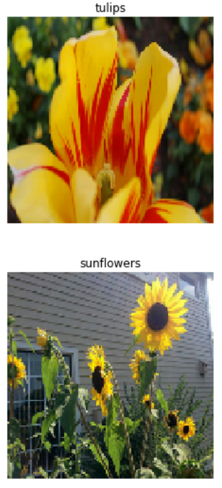
실제 환경의 이미지 데이터를 학습시킬 때, 보통 서로 다른 크기의 이미지를 공통 크기로 변환하여 고정 크기의 배치를 사용합니다. flower 데이터셋을 사용해봅시다.

list_ds = tf.data.Dataset.list_files(str(flowers_root/'*/*'))

다음 함수는 데이터셋을 적절하게 처리합니다.

# Reads an image from a file, decodes it into a dense tensor, and resizes it
# to a fixed shape.
def parse_image(filename):
  parts = tf.strings.split(filename, '/')
  label = parts[-2]

  image = tf.io.read_file(filename)
  image = tf.image.decode_jpeg(image)
  image = tf.image.convert_image_dtype(image, tf.float32)
  image = tf.image.resize(image, [128, 128])
  return image, label
  • io.read_file: 파일을 읽은 뒤,
  • decode_jped: 이미지 파일을 디코딩합니다.
  • convert_image_dtype: 이미지의 타입을 tf.float32로 변환하고,
  • tf.image.resize: [128, 128]의 크기로 이미지 크기를 변환합니다.

실험해보죠.

file_path = next(iter(list_ds))
image, label = parse_image(file_path)

def show(image, label):
  plt.figure()
  plt.imshow(image)
  plt.title(label.numpy().decode('utf-8'))
  plt.axis('off')

show(image, label)

map 함수를 이용해서 데이터셋에 적용해보죠.

images_ds = list_ds.map(parse_image)

for image, label in images_ds.take(2):
  show(image, label)

Applying arbitrary Python logic

데이터 전처리 작업에 TensorFlow 연산을 사용하면 성능적으로 이득을 볼 수 있습니다. 하지만 가끔은 입력 데이터를 처리하기 위해 파이썬 라이브러리 함수가 유용할 때가 있습니다. 이를 위해 Dataset.map()에서 tf.py_function()을 사용하세요.

예를 들어, random rotation 처리를 적용하고 싶지만 TensorFlow 연산은 tf.imagetf.image.rot90 함수만 제공하기 때문에 유용하지 않을 수 있습니다. tf.py_function()을 경험해보기 위해, scipy.ndimage.rotate 함수를 사용해보죠.

import scipy.ndimage as ndimage

def random_rotate_image(image):
  image = ndimage.rotate(image, np.random.uniform(-30, 30), reshape=False)
  return image
image, label = next(iter(images_ds))
image = random_rotate_image(image)
show(image, label)

이 함수를 Dataset.map() 함수와 함께 사용하려면 Dataset.from_generator처럼 shape과 type을 명시해주어야 합니다.

def tf_random_rotate_image(image, label):
  im_shape = image.shape
  [image,] = tf.py_function(random_rotate_image, [image], [tf.float32])
  image.set_shape(im_shape)
  return image, label
  • shape는 set_shape, type은 tf.py_function의 [tf.float32]를 통해 명시해주는 것 같습니다.
rot_ds = images_ds.map(tf_random_rotate_image)

for image, label in rot_ds.take(2):
  show(image, label)
  • images_ds는 flower dataset에서 이미지의 크기를 [128, 128]로 변환하여 반환하는 객체입니다.

Parsing tf.Example protocol buffer messages

많은 입력 파이프라인이 TFRecord 형식에서 tf.train.Example 프로토콜 버퍼 메시지를 추출합니다. tf.train.Example은 하나 또는 그 이상의 "특성"을 가지고, 입력 파이프라인은 이러한 특성을 텐서로 변환하여 사용합니다.

fsns_test_file = tf.keras.utils.get_file("fsns.tfrec", "https://storage.googleapis.com/download.tensorflow.org/data/fsns-20160927/testdata/fsns-00000-of-00001")
dataset = tf.data.TFRecordDataset(filenames = [fsns_test_file])
dataset
  • <TFRecordDatasetV2 shapes: (), types: tf.string>

tf.train.Example 프로토를 사용하여 tf.data.Dataset의 데이터를 확인할 수 있습니다.

raw_example = next(iter(dataset))
parsed = tf.train.Example.FromString(raw_example.numpy())

feature = parsed.features.feature
raw_img = feature['image/encoded'].bytes_list.value[0]
img = tf.image.decode_png(raw_img)
plt.imshow(img)
plt.axis('off')
_ = plt.title(feature["image/text"].bytes_list.value[0])

  • tf.train.Example.FromString을 통해 feature를 읽어오고, feature의 ['image/encoded']는 이미지, ["image/text"]는 해당 이미지의 레이블을 의미하는 것 같습니다.
raw_example = next(iter(dataset))

def tf_parse(eg):
  example = tf.io.parse_example(
      eg[tf.newaxis], {
          'image/encoded': tf.io.FixedLenFeature(shape=(), dtype=tf.string),
          'image/text': tf.io.FixedLenFeature(shape=(), dtype=tf.string)
      })
  return example['image/encoded'][0], example['image/text'][0]
  
img, txt = tf_parse(raw_example)
print(txt.numpy())
print(repr(img.numpy()[:20]), "...")
  • b'Rue Perreyon'
    b'\x89PNG\r\n\x1a\n\x00\x00\x00\rIHDR\x00\x00\x02X' ...
  • tf.io.FixedLenFeature 함수는 고정길이의 입력 특성을 가져옵니다.
decoded = dataset.map(tf_parse)
decoded
  • <MapDataset shapes: ((), ()), types: (tf.string, tf.string)>
image_batch, text_batch = next(iter(decoded.batch(10)))
image_batch.shape
  • TensorShape([10])

Time series windowing

end-to-end 시계열 예시는 다음을 참조하세요.

시계열 데이터는 시간축을 변형하지 않고 그대로 사용합니다. Dataset.range를 사용해서 이를 확인해보죠.

range_ds = tf.data.Dataset.range(100000)

일반적으로 이러한 종류를 사용하는 모델은 연속적인 시간 단위를 사용할 것입니다.(예를 들면, 주 단위, 일 단위, 월 단위 또는 기타 등등) 가장 간단한 방법은 역시 배치 형태로 사용하는 것입니다.

Using batch

batches = range_ds.batch(10, drop_remainder=True)

for batch in batches.take(5):
  print(batch.numpy())
  • [0 1 2 3 4 5 6 7 8 9]
    [10 11 12 13 14 15 16 17 18 19]
    [20 21 22 23 24 25 26 27 28 29]
    [30 31 32 33 34 35 36 37 38 39]
    [40 41 42 43 44 45 46 47 48 49]
  • drop_remainder는 마지막 배치를 무시하는 인자입니다.

또는, dense한 prediction을 원할 경우, feature와 label을 한 단계씩 이동(shift)할 수 있습니다.

def dense_1_step(batch):
  # Shift features and labels one step relative to each other.
  return batch[:-1], batch[1:]

predict_dense_1_step = batches.map(dense_1_step)

for features, label in predict_dense_1_step.take(3):
  print(features.numpy(), " => ", label.numpy())
  • [0 1 2 3 4 5 6 7 8]  =>  [1 2 3 4 5 6 7 8 9]
    [10 11 12 13 14 15 16 17 18]  =>  [11 12 13 14 15 16 17 18 19]
    [20 21 22 23 24 25 26 27 28]  =>  [21 22 23 24 25 26 27 28 29]
batches = range_ds.batch(15, drop_remainder=True)

def label_next_5_steps(batch):
  return (batch[:-5],   # Take the first 5 steps
          batch[-5:])   # take the remainder

predict_5_steps = batches.map(label_next_5_steps)

for features, label in predict_5_steps.take(3):
  print(features.numpy(), " => ", label.numpy())
  • 데이터셋은 15 배치 크기를 가집니다. label_next_5_steps에서 batch[:-5]는 학습 데이터로 0~9까지 10개, batch[-5:]는 레이블로 10~14까지 5개를 반환합니다.
  • [0 1 2 3 4 5 6 7 8 9]  =>  [10 11 12 13 14]
    [15 16 17 18 19 20 21 22 23 24]  =>  [25 26 27 28 29]
    [30 31 32 33 34 35 36 37 38 39]  =>  [40 41 42 43 44]

데이터셋의 특성과 레이블이 각 배치에서 오버래핑하기 위해 Dataset.zip을 사용하세요.

feature_length = 10
label_length = 5

features = range_ds.batch(feature_length, drop_remainder=True)
labels = range_ds.batch(feature_length).skip(1).map(lambda labels: labels[:-5])

predict_5_steps = tf.data.Dataset.zip((features, labels))

for features, label in predict_5_steps.take(3):
  print(features.numpy(), " => ", label.numpy())
  • [0 1 2 3 4 5 6 7 8 9]  =>  [10 11 12 13 14]
    [10 11 12 13 14 15 16 17 18 19]  =>  [20 21 22 23 24]
    [20 21 22 23 24 25 26 27 28 29]  =>  [30 31 32 33 34]

Using window

Dataset.batch 작업을 사용하는 동안, 세부적인 통제가 필요한 상황이 있을 수 있습니다. Dataset.window는 이러한 작업을 수행할 수 있도록 합니다. 대신, DatasetsDataset을 반환합니다. 자세한 사항은 다음을 참조하세요.

window_size = 5

windows = range_ds.window(window_size, shift=1)
for sub_ds in windows.take(5):
  print(sub_ds)
  • <_VariantDataset shapes: (), types: tf.int64>
    <_VariantDataset shapes: (), types: tf.int64>
    <_VariantDataset shapes: (), types: tf.int64>
    <_VariantDataset shapes: (), types: tf.int64>
    <_VariantDataset shapes: (), types: tf.int64>

Dataset.flat_map 함수는 datasets의 dataset을 가져와서 단일 dataset으로 만들 수 있습니다.

 for x in windows.flat_map(lambda x: x).take(30):
   print(x.numpy(), end=' ')
  • 0 1 2 3 4 1 2 3 4 5 2 3 4 5 6 3 4 5 6 7 4 5 6 7 8 5 6 7 8 9
  • windows는 [0, 1, 2, 3, 4] --> [1, 2, 3, 4, 5] --> [2, 3, 4, 5, 6] --> ... 과 같이 데이터를 반환합니다.

거의 모든 경우에서, dataset의 첫 단계로 .batch를 사용할 것입니다.

def sub_to_batch(sub):
  return sub.batch(window_size, drop_remainder=True)

for example in windows.flat_map(sub_to_batch).take(5):
  print(example.numpy())
  • [0 1 2 3 4]
    [1 2 3 4 5]
    [2 3 4 5 6]
    [3 4 5 6 7]
    [4 5 6 7 8]

shift 인자가 이동 크기를 제어할 수 있습니다. 다음 예는 이를 보여줍니다.

def make_window_dataset(ds, window_size=5, shift=1, stride=1):
  windows = ds.window(window_size, shift=shift, stride=stride)

  def sub_to_batch(sub):
    return sub.batch(window_size, drop_remainder=True)

  windows = windows.flat_map(sub_to_batch)
  return windows
ds = make_window_dataset(range_ds, window_size=10, shift = 5, stride=3)

for example in ds.take(10):
  print(example.numpy())
  • [ 0  3  6  9 12 15 18 21 24 27]
    [ 5  8 11 14 17 20 23 26 29 32]
    [10 13 16 19 22 25 28 31 34 37]
    [15 18 21 24 27 30 33 36 39 42]
    [20 23 26 29 32 35 38 41 44 47]
    [25 28 31 34 37 40 43 46 49 52]
    [30 33 36 39 42 45 48 51 54 57]
    [35 38 41 44 47 50 53 56 59 62]
    [40 43 46 49 52 55 58 61 64 67]
    [45 48 51 54 57 60 63 66 69 72
  • shift는 각 리스트의 맨 앞의 값을 보면 알 수 있고, stride는 리스트 안의 각 값의 차이를 보면 알 수 있습니다.

이제 레이블을 좀 더 쉽게 추출할 수 있습니다.

dense_labels_ds = ds.map(dense_1_step)

for inputs,labels in dense_labels_ds.take(3):
  print(inputs.numpy(), "=>", labels.numpy())
  • [ 0  3  6  9 12 15 18 21 24] => [ 3  6  9 12 15 18 21 24 27]
    [ 5  8 11 14 17 20 23 26 29] => [ 8 11 14 17 20 23 26 29 32]
    [10 13 16 19 22 25 28 31 34] => [13 16 19 22 25 28 31 34 37]
  • dense_1_step은 batch[-1:], batch[1:]를 반환하는 함수입니다.

Resampling


class-imbalanced한 작업을 수행할 때, dataset을 적절한 방법으로 샘플링해야 합니다. tf.data는 이를 위한 두 가지 방법을 제공합니다. 신용카드 이상탐지 데이터셋은 이 문제를 다루기 위한 매우 좋은 예제입니다.

zip_path = tf.keras.utils.get_file(
    origin='https://storage.googleapis.com/download.tensorflow.org/data/creditcard.zip',
    fname='creditcard.zip',
    extract=True)

csv_path = zip_path.replace('.zip', '.csv')
creditcard_ds = tf.data.experimental.make_csv_dataset(
    csv_path, batch_size=1024, label_name="Class",
    # Set the column types: 30 floats and an int.
    column_defaults=[float()]*30+[int()])

클래스 분포를 확인합니다. 매우 비대칭적입니다.(skewed)

def count(counts, batch):
  features, labels = batch
  class_1 = labels == 1
  class_1 = tf.cast(class_1, tf.int32)

  class_0 = labels == 0
  class_0 = tf.cast(class_0, tf.int32)

  counts['class_0'] += tf.reduce_sum(class_0)
  counts['class_1'] += tf.reduce_sum(class_1)

  return counts
counts = creditcard_ds.take(10).reduce(
    initial_state={'class_0': 0, 'class_1': 0},
    reduce_func = count)

counts = np.array([counts['class_0'].numpy(),
                   counts['class_1'].numpy()]).astype(np.float32)

fractions = counts/counts.sum()
print(fractions)
  • reduce 함수는 데이터의 각 요소에 단일 함수를 적용하는 함수입니다.

tf.data는 class-imbalanced 문제를 해결하기 위한 몇 가지 방법을 제공합니다.

Datasets sampling

첫 번째 방법은 sample_from_datasets를 활용하는 것입니다. data.Dataset의 각 클래스를 분리할 때 매우 유용합니다.

필터를 사용해서 신용카드 이상탐지 데이터를 생성합니다.

negative_ds = (
  creditcard_ds
    .unbatch()
    .filter(lambda features, label: label==0)
    .repeat())
positive_ds = (
  creditcard_ds
    .unbatch()
    .filter(lambda features, label: label==1)
    .repeat())
for features, label in positive_ds.batch(10).take(1):
  print(label.numpy())
  • [1 1 1 1 1 1 1 1 1 1]

tf.data.experimental.sample_from_datasets에 데이터를 통과시키고, 가중을 부과할 수 있습니다.

balanced_ds = tf.data.experimental.sample_from_datasets(
    [negative_ds, positive_ds], [0.5, 0.5]).batch(10)

다음과 같이 50:50의 확률로 클래스를 생성합니다.

for features, labels in balanced_ds.take(10):
  print(labels.numpy())
  • [0 0 1 1 0 0 1 1 1 1]
    [0 0 0 0 1 1 1 1 0 0]
    [0 0 0 0 0 0 1 0 1 1]
    [1 0 1 1 0 0 0 0 1 0]
    [0 1 0 1 0 1 1 0 1 0]
    [1 0 0 1 0 1 1 0 1 0]
    [0 1 1 1 0 0 1 0 1 1]
    [1 0 0 1 0 0 1 0 0 0]
    [1 0 0 1 0 0 0 1 0 1]
    [1 1 0 1 1 0 1 1 1 0]

Rejection resampling

먼저, rejection resampling은 리샘플링에서도 자주 사용되는 방법입니다. 이에 대해 관심이 있다면, 직접 검색하여 공부하는 것도 나쁘지 않습니다.

experimental.sample_from_datasets의 문제점은 클래스마다 별도의 tf.data.Dataset가 필요하다는 것입니다. Dataset.filter를 사용하면 해결할 수 있지만, 데이터를 두배로 로드하는 결과를 초래합니다.

data.experimental.rejection_resample 함수는 dataset 한 번만 로드하여 균형잡힌 결과를 얻을 수 있게 도와줍니다. 밸런스를 위해 이에 위반하는 요소는 제거됩니다. data.experimental.rejection_resample에서 class_func 인자를 사용합니다. class_func 인자는 각 dataset의 요소에 적용되며, 밸런싱을 위해 어떤 클래스에 속하는지를 결정합니다.

creditcard_ds의 요소는 (features, label) 쌍으로 이루어져 있습니다. class_func는 해당 레이블을 반환합니다.

def class_func(features, label):
  return label

resampler는 target distribution을 필요로 하며, 선택적으로 initial distribution 추정을 필요로 합니다.

resampler = tf.data.experimental.rejection_resample(
    class_func, target_dist=[0.5, 0.5], initial_dist=fractions)

resampler는 개별 요소를 다루기 때문에, unbatch를 통해 배치를 해제해야 합니다.

resample_ds = creditcard_ds.unbatch().apply(resampler).batch(10)

resampler는 class_func의 출력값으로 (class, example) 쌍을 반환합니다. 이 경우, example이 이미 (feature, label) 쌍을 이루고 있으므로, 중복되는 레이블은 제거하도록 합시다(여기서 class를 의미합니다).

balanced_ds = resample_ds.map(lambda extra_label, features_and_label: features_and_label)

dataset은 각 클래스를 50:50 비율로 생성합니다.

for features, labels in balanced_ds.take(10):
  print(labels.numpy())
  • [0 1 0 1 0 1 0 0 0 0]
    [1 0 1 1 1 1 0 0 1 1]
    [0 1 1 1 0 0 1 1 1 0]
    [1 1 0 1 0 0 0 1 0 0]
    [0 0 0 0 1 1 0 0 1 1]
    [0 1 1 0 0 1 0 1 0 1]
    [1 1 1 0 0 0 1 0 1 0]
    [1 0 1 1 1 1 1 1 1 0]
    [1 1 1 1 0 1 0 1 0 1]
    [1 0 0 0 0 0 1 1 0 1]