Warm-up 방식의 학습 방법, 학습률을 높였다가 낮췄다가, 다시 높였다가 낮췄다가 등 학습 과정에서 다양한 학습률로 local optima를 빠져나오도록 장치하는 방법이 fixed learning rate 방법보다 성능이 더 좋다는 것은 이미 오래전부터 논문을 통해 증명되어 왔습니다.
Cosine Annealing을 사용하면 learning rate가 어떻게 변하는지 알아보겠습니다.
설명하는 코드는 케라스 콜백과 같이 등록하여 사용하면 됩니다.
import tensorflow as tf
import tensorflow.keras.backend as backend
import math

# CosineAnneling Example.
class CosineAnnealingLearningRateSchedule(tf.keras.callbacks.Callback):
    # constructor
    def __init__(self, n_epochs, n_cycles, lrate_max, min_lr, verbose = 0):
        self.epochs = n_epochs
        self.cycles=  n_cycles
        self.lr_max = lrate_max
        self.min_lr = min_lr
        self.lrates = list()

    # caculate learning rate for an epoch
    def cosine_annealing(self, epoch, n_epochs, n_cycles, lrate_max):
        # 전체 epoch / 설정 cycle 수만큼 cycle을 반복합니다.
        epochs_per_cycle = math.floor(n_epochs/n_cycles)
        cos_inner = (math.pi * (epoch % epochs_per_cycle)) / (epochs_per_cycle)

        return lrate_max/2 * (math.cos(cos_inner) + 1)

    # calculate and set learning rate at the start of the epoch
    def on_epoch_begin(self, epoch, logs = None):
        if(epoch < 101):
            # calculate learning rate
            lr = self.cosine_annealing(epoch, self.epochs, self.cycles, self.lr_max)
            print('\nEpoch %05d: CosineAnnealingScheduler setting learng rate to %s.' % (epoch + 1, lr))
        # 101번째 epoch부터는 해당 설정한 min_lr을 사용
        else:
            lr = self.min_lr

        #     elif((epoch >= 65) and (epoch < 75)):
        #       lr = 1e-5
        #       print('\n No CosineAnnealingScheduler set lr 1e-5')
        #     elif((epoch >= 75) and (epoch < 85)):
        #       lr = 1e-6
        #       print('\n No CosineAnnealingScheduler set lr 1e-6')
        #     elif((epoch >= 85)):
        #       lr = 1e-7
        #       print('\n No CosineAnnealingScheduler set lr 1e-7')

        # set learning rate
        # 아래 예제 코드 실행을 위해선 밑 코드를 주석 처리 해주세요.
        backend.set_value(self.model.optimizer.lr, lr)
        # log value
        self.lrates.append(lr)
위 코드를 사용하면, 아래와 같은 학습률 변화를 볼 수 있습니다.
cosine_schedule = CosineAnnealingLearningRateSchedule(n_epochs = 100, n_cycles = 5, lrate_max = 1e-3, min_lr = 1e-6)

for i in range(1, 100 + 1):
    cosine_schedule.on_epoch_begin(i)

import matplotlib.pyplot as plt

plt.plot(cosine_schedule.lrates)
plt.title('Cosine Annealing_Toy')
plt.xlabel('epochs'); plt.ylabel('learning_rate')
plt.grid()
plt.show()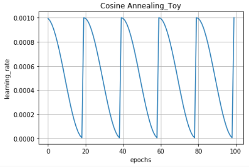
n_cycle을 5로 지정한만큼, 20(100/5) 수를 기준으로 cycle이 반복되고 있습니다.
사실 텐서플로우를 사용한다면 위처럼 직접 정의하여 사용하지 않아도 됩니다.
텐서플로우 공식 홈페이지를 보면 이미 학습률을 조절할 수 있는 다양한 방법들을 제공하고 있기 때문에 가져다 사용하면 됩니다.
(CosineDecayRestarts, CosineDecay 등)
다음 글에서는 텐서플로우에서 제공하는 함수를 사용하여 MNIST 데이터셋에 적용해보겠습니다.
'# Machine Learning > Keras Implementation' 카테고리의 다른 글
| Tensorflow Gradient Accumulation 간단 구현 (1) | 2021.07.18 |
|---|---|
| Albumentation 사용해서 Augmentation하기 (0) | 2020.08.25 |
| keras load_model(), 커스텀 객체를 포함한 모델을 로드해보자 (0) | 2020.07.10 |
| 케라스 layer 시각화하기 (visualization) (0) | 2020.03.27 |
| keras custom generator - 2 (0) | 2020.01.31 |