이글은 다음 문서를 참조합니다.
www.tensorflow.org/guide/keras/functional
(번역은 자력 + 파파고 + 구글 번역기를 사용하였으니, 부자연스럽더라도 양해바랍니다.)
The Keras Functional API in Tensorflow
!pip install -q pydot
!pip install graphviz(apt-get install graphviz)
pydot, graphviz를 설치해줍니다. 나중에 model_plot 그릴때 사용됩니다. (graphviz import error 는 밑쪽에)
Introduction
우리는 이미 keras.Sequential()을 이용하여 모델 만들기에 익숙해져있습니다. 함수형 API는 Sequential을 통한 모델 생성보다 더 유연하게 모델을 구축할 수 있습니다: 비선형 구조, 층 공유, 다중 입출력 모델을 다룰 수 있습니다.
딥러닝은 DAG(directed acyclic graph) 아이디어로 구성되어있다. 함수형 API는 층에 대한 그래프를 만들기 위한 도구이다.
다음 모델을 고려해보자:
(input: 784-dimensional vectors)
       ↧
[Dense (64 units, relu activation)]
       ↧
[Dense (64 units, relu activation)]
       ↧
[Dense (10 units, softmax activation)]
       ↧
(output: probability distribution over 10 classes)
3개의 단순한 층으로 이루어진 그래프이다.
함수형 API로는 다음과 같이 만들 수 있고, 입력 노드는 다음과 같다.
from tensorflow import keras

inputs = keras.Input(shape=(784,))
우리의 데이터가 784차원임을 나타내준다. 배치 크기가 항상 생략할 수 있고, 우리는 그저 각 데이터의 구체적인 shape만 알려주면 된다. 만약 데이터가 (32, 32, 3)으로 이루어져 있다면 다음과 같을 것이다.
img_inputs = keras.Input(shape=(32, 32, 3))
Input 함수의 반환은 input data의 dtype과 shape에 관한 정보를 포함합니다.
inputs.shape = TensorShape([None, 784])
inputs.dtype = tf.float32
층 그래프에 inputs object로 새로운 노드를 다음과 같이 만들 수 있습니다.
(층 그래프란 것은 쉽게 말해서 텐서플로우에서 Session안에 층을 구성하면 한 그래프에 층이 쌓이게(stack) 됩니다. 그래프는 통이고 층은 내용물이라고 생각하면 쉽겠네요.)
from tensorflow.keras import layers

dense = layers.Dense(64, activation='relu')
x = dense(inputs)
"layer call"은 우리가 만든 layer로 inputs에서 화살표를 그리는 것과 같습니다. dense layer에 입력을 통과시키고 x를 얻습니다.
더 추가해봅시다.
x = layers.Dense(64, activation='relu')(x)
outputs = layers.Dense(10, activation='softmax')(x)
입력과 출력을 지정하여 Model을 만들 수 있습니다.
model = keras.Model(inputs=inputs, outputs=outputs)
복습합시다. 전체 과정은 다음과 같습니다.
inputs = keras.Input(shape=(784,), name='img')
x = layers.Dense(64, activation='relu')(inputs)
x = layers.Dense(64, activation='relu')(x)
outputs = layers.Dense(10, activation='softmax')(x)

model = keras.Model(inputs=inputs, outputs=outputs, name='mnist_model')
여러분이 만든 모델은 model.summary()를 이용하여 파라미터 수와 층이 어떻게 구성되어있는지 확인할 수 있습니다.
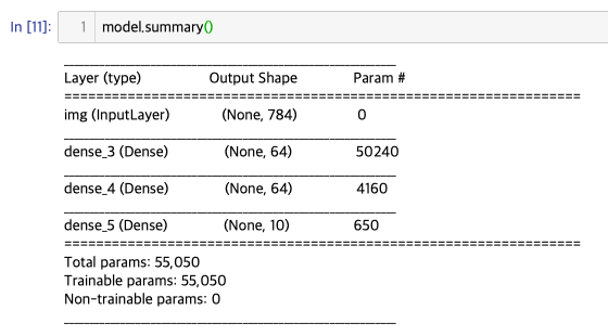
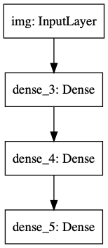
또한, keras.utils.plot_model(model, 'my_first_model.png')를 사용하면 예쁘게 그림도 그려주고 저장도 해줍니다.
ImportError: You must install pydot and graphviz for `pydotprint` to work.
-> 저는 pip말고 brew install graphviz로 설치하니까 되더군요.
선택적으로 shape도 보여줍니다.
keras.utils.plot_model(model, 'my_first_model_with_shape_info.png', show_shapes=True)
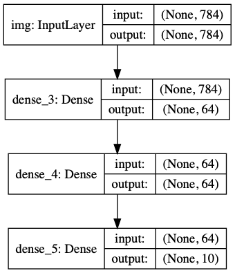
이러한 그림들과 코드는 사실상 동일함을 나타냅니다. 코드에서 연결화살표는 함수 호출을 의미합니다.
"graph of layers"는 딥러닝 모델을 직관적으로 나타내는 이미지이며, 함수형 API는 이러한 것을 나타내는데 도움을 줍니다.
Training, evaluation, and inference
훈련, 평가, 추론은 Sequential 모델에서 작동하듯이 함수형 API에서도 똑같이 작동합니다.
바로 예시를 보죠.
MNIST 데이터가 있고, validation_spilit을 통해 모니터링하면서 fit시킨 후 평가합니다.
(x_train, y_train), (x_test, y_test) = keras.datasets.mnist.load_data()
x_train = x_train.reshape(60000, 784).astype('float32') / 255
x_test = x_test.reshape(10000, 784).astype('float32') / 255

model.compile(loss='sparse_categorical_crossentropy',
              optimizer=keras.optimizers.RMSprop(),
              metrics=['accuracy'])
history = model.fit(x_train, y_train,
                    batch_size=64,
                    epochs=5,
                    validation_split=0.2)
test_scores = model.evaluate(x_test, y_test, verbose=0)
print('Test loss:', test_scores[0])
print('Test accuracy:', test_scores[1])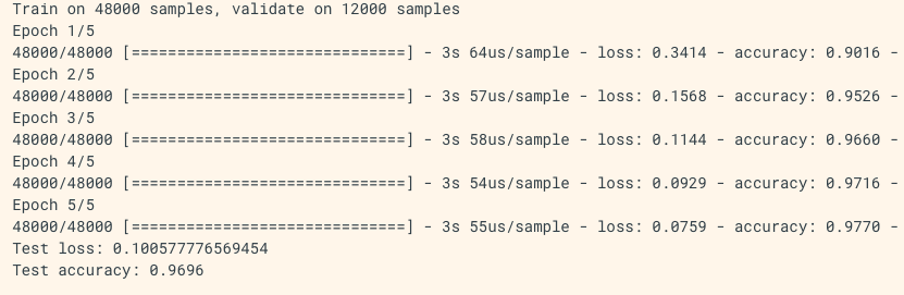
Saving and Serialization
이 기능 또한 함수형 API에서도 사용할 수 있습니다.
model.save() 를 통해 모델을 저장할 수 있고, 코드가 있지 않아도 같은 구조의 모델을 load할 수 있습니다.
이 파일에는 다음과 같은 내용이 포함됨: - 모델의 아키텍처 - 모델의 weights 값(교육 중에 학습됨) - 모델의 training config(model.compile) 구성(편집하기 위해 전달된 내용), 있는 경우 - optimizer와 해당 상태(이 경우, 중단한 곳에서 교육을 다시 시작할 수 있음)
model.save('path_to_my_model.h5')
del model
# Recreate the exact same model purely from the file:
model = keras.models.load_model('path_to_my_model.h5')
Using the same graph of layers to define multiple models
함수형 API는 구체적으로 입출력을 지정할 수 있습니다. 이는 다중 입출력 모델 또한 구성 가능하다는 것을 뜻합니다.
아래 예시는 2 Model로 auto-encoder를 구성하는 것을 나타냅니다.
encoder_input = keras.Input(shape=(28, 28, 1), name='img')
x = layers.Conv2D(16, 3, activation='relu')(encoder_input)
x = layers.Conv2D(32, 3, activation='relu')(x)
x = layers.MaxPooling2D(3)(x)
x = layers.Conv2D(32, 3, activation='relu')(x)
x = layers.Conv2D(16, 3, activation='relu')(x)
encoder_output = layers.GlobalMaxPooling2D()(x)

encoder = keras.Model(encoder_input, encoder_output, name='encoder')
encoder.summary()

x = layers.Reshape((4, 4, 1))(encoder_output)
x = layers.Conv2DTranspose(16, 3, activation='relu')(x)
x = layers.Conv2DTranspose(32, 3, activation='relu')(x)
x = layers.UpSampling2D(3)(x)
x = layers.Conv2DTranspose(16, 3, activation='relu')(x)
decoder_output = layers.Conv2DTranspose(1, 3, activation='relu')(x)

autoencoder = keras.Model(encoder_input, decoder_output, name='autoencoder')
autoencoder.summary()
(꼭 summary()를 확인하세요!)
이러한 구성은 input_shape를 가진 output을 만들어내기 위해 필요합니다.
Conv2D의 반대는 Conv2DTranspose(가중치 학습 가능), MaxPooling2D의 받내는 UpSampling2D(가중치 학습 x)
All models are callable, just like layers
어떠한 모델이던 다른 층의 출력이나 입력을 층으로서 활용이 가능합니다. 이때, 모델 구조를 재사용하는 것이 아닌 가중치를 재사용한다는 것을 명심하세요
encoder_input = keras.Input(shape=(28, 28, 1), name='original_img')
x = layers.Conv2D(16, 3, activation='relu')(encoder_input)
x = layers.Conv2D(32, 3, activation='relu')(x)
x = layers.MaxPooling2D(3)(x)
x = layers.Conv2D(32, 3, activation='relu')(x)
x = layers.Conv2D(16, 3, activation='relu')(x)
encoder_output = layers.GlobalMaxPooling2D()(x)

encoder = keras.Model(encoder_input, encoder_output, name='encoder')
encoder.summary()

decoder_input = keras.Input(shape=(16,), name='encoded_img')
x = layers.Reshape((4, 4, 1))(decoder_input)
x = layers.Conv2DTranspose(16, 3, activation='relu')(x)
x = layers.Conv2DTranspose(32, 3, activation='relu')(x)
x = layers.UpSampling2D(3)(x)
x = layers.Conv2DTranspose(16, 3, activation='relu')(x)
decoder_output = layers.Conv2DTranspose(1, 3, activation='relu')(x)

decoder = keras.Model(decoder_input, decoder_output, name='decoder')
decoder.summary()

autoencoder_input = keras.Input(shape=(28, 28, 1), name='img')
encoded_img = encoder(autoencoder_input)
decoded_img = decoder(encoded_img)
autoencoder = keras.Model(autoencoder_input, decoded_img, name='autoencoder')
autoencoder.summary()
(꼭 summary()를 확인하세요!)
모델 앙상블링은 다음과 같이 구성됩니다.
def get_model():
  inputs = keras.Input(shape=(128,))
  outputs = layers.Dense(1, activation='sigmoid')(inputs)
  return keras.Model(inputs, outputs)

model1 = get_model()
model2 = get_model()
model3 = get_model()

inputs = keras.Input(shape=(128,))
y1 = model1(inputs)
y2 = model2(inputs)
y3 = model3(inputs)
outputs = layers.average([y1, y2, y3])
ensemble_model = keras.Model(inputs=inputs, outputs=outputs)
Manipulating complex graph topologies
Models with multiple inputs and outputs
함수형 API는 다중 입출력을 구성할 수 있습니다.
다음 예제를 보겠습니다.
티켓 우선순위에 따라 올바른 부서에 전달하는 시스템을 구축하고 있다고 생각합시다.
우리는 3개의 input을 가집니다.
- Title of the ticket (text input)
- Text body of the ticket (text input)
- Any tags added by the user (categorical input)
또한, 2가지 output을 가집니다.
- Priority score between 0 and 1 (scalar sigmoid output)
- The department that should handle the ticket (softmax output over the set of departments)
코드를 볼까요.
num_tags = 12  # Number of unique issue tags
num_words = 10000  # Size of vocabulary obtained when preprocessing text data
num_departments = 4  # Number of departments for predictions

title_input = keras.Input(shape=(None,), name='title')  # Variable-length sequence of ints
body_input = keras.Input(shape=(None,), name='body')  # Variable-length sequence of ints
tags_input = keras.Input(shape=(num_tags,), name='tags')  # Binary vectors of size `num_tags`

# Embed each word in the title into a 64-dimensional vector
title_features = layers.Embedding(num_words, 64)(title_input)
# Embed each word in the text into a 64-dimensional vector
body_features = layers.Embedding(num_words, 64)(body_input)

# Reduce sequence of embedded words in the title into a single 128-dimensional vector
title_features = layers.LSTM(128)(title_features)
# Reduce sequence of embedded words in the body into a single 32-dimensional vector
body_features = layers.LSTM(32)(body_features)

# Merge all available features into a single large vector via concatenation
x = layers.concatenate([title_features, body_features, tags_input])

# Stick a logistic regression for priority prediction on top of the features
priority_pred = layers.Dense(1, activation='sigmoid', name='priority')(x)
# Stick a department classifier on top of the features
department_pred = layers.Dense(num_departments, activation='softmax', name='department')(x)

# Instantiate an end-to-end model predicting both priority and department
model = keras.Model(inputs=[title_input, body_input, tags_input],
                    outputs=[priority_pred, department_pred])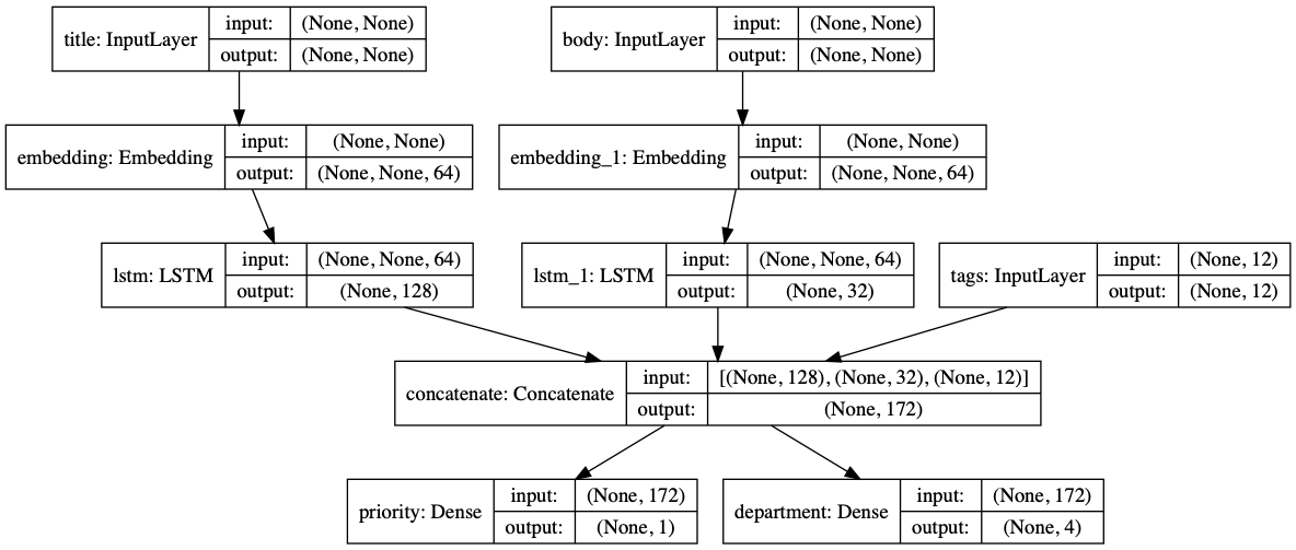
loss 또한, 각각 output에 대해 적절한 함수를 적용할 수 있습니다.
추가로 가중치를 줘서 각각 loss값이 total loss에 미치는 영향도를 조절할 수도 있습니다.
model.compile(optimizer=keras.optimizers.RMSprop(1e-3),
              loss=['binary_crossentropy', 'categorical_crossentropy'],
              loss_weights=[1., 0.2])
이름도 붙여 줄 수 있습니다.
model.compile(optimizer=keras.optimizers.RMSprop(1e-3),
              loss={'priority': 'binary_crossentropy',
                    'department': 'categorical_crossentropy'},
              loss_weights=[1., 0.2])
넘파이 배열을 이용하여 fit 시켜보겠습니다.
import numpy as np

# Dummy input data
title_data = np.random.randint(num_words, size=(1280, 10))
body_data = np.random.randint(num_words, size=(1280, 100))
tags_data = np.random.randint(2, size=(1280, num_tags)).astype('float32')
# Dummy target data
priority_targets = np.random.random(size=(1280, 1))
dept_targets = np.random.randint(2, size=(1280, num_departments))

model.fit({'title': title_data, 'body': body_data, 'tags': tags_data},
          {'priority': priority_targets, 'department': dept_targets},
          epochs=2,
          batch_size=32)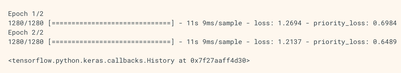
data, label을 fit시킬 떄는 두 가지 방법이 가능합니다.
- ([title_data, body_data, tags_data], [priority_targets, dept_targets])
- ({'title': title_data, 'body': body_data, 'tags': tags_data}, {'priority': priority_targets, 'department': dept_targets})
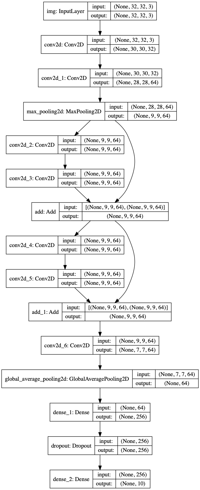
A toy resnet model
함수형 API는 resnet과 같은 비선형적 모델 구조를 구성하기 쉽습니다.
잔차 연결의 예시를 봅시다.
inputs = keras.Input(shape=(32, 32, 3), name='img')
x = layers.Conv2D(32, 3, activation='relu')(inputs)
x = layers.Conv2D(64, 3, activation='relu')(x)
block_1_output = layers.MaxPooling2D(3)(x)

x = layers.Conv2D(64, 3, activation='relu', padding='same')(block_1_output)
x = layers.Conv2D(64, 3, activation='relu', padding='same')(x)
block_2_output = layers.add([x, block_1_output])

x = layers.Conv2D(64, 3, activation='relu', padding='same')(block_2_output)
x = layers.Conv2D(64, 3, activation='relu', padding='same')(x)
block_3_output = layers.add([x, block_2_output])

x = layers.Conv2D(64, 3, activation='relu')(block_3_output)
x = layers.GlobalAveragePooling2D()(x)
x = layers.Dense(256, activation='relu')(x)
x = layers.Dropout(0.5)(x)
outputs = layers.Dense(10, activation='softmax')(x)

model = keras.Model(inputs, outputs, name='toy_resnet')
model.summary()
(꼭 summary()를 확인하세요!)
train 시켜 보겠습니다.
(x_train, y_train), (x_test, y_test) = keras.datasets.cifar10.load_data()
x_train = x_train.astype('float32') / 255.
x_test = x_test.astype('float32') / 255.
y_train = keras.utils.to_categorical(y_train, 10)
y_test = keras.utils.to_categorical(y_test, 10)

model.compile(optimizer=keras.optimizers.RMSprop(1e-3),
              loss='categorical_crossentropy',
              metrics=['acc'])
model.fit(x_train, y_train,
          batch_size=64,
          epochs=1,
          validation_split=0.2)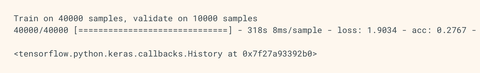
Sharing layers
함수형 API는 공유 층을 사용하기에도 좋습니다.
밑의 예시는 한가지 임베딩 층에 두가지 입력을 넣어 재사용성을 높였고, 여러 입력을 학습합니다.
공유 계층은 이러한 서로 다른 입력에 걸친 정보의 공유를 가능하게 하고, 그러한 모형을 더 적은 데이터로 훈련시킬 수 있게 하기 때문에 유사한 공간(예: 유사한 어휘를 특징으로 하는 두 개의 다른 텍스트)에서 오는 입력을 인코딩하는 데 자주 사용된다. 입력 중 하나에서 특정 단어가 보이는 경우, 공유 계층을 통과하는 모든 입력의 처리에 도움이 될 것이다.
# Embedding for 1000 unique words mapped to 128-dimensional vectors
shared_embedding = layers.Embedding(1000, 128)

# Variable-length sequence of integers
text_input_a = keras.Input(shape=(None,), dtype='int32')

# Variable-length sequence of integers
text_input_b = keras.Input(shape=(None,), dtype='int32')

# We reuse the same layer to encode both inputs
encoded_input_a = shared_embedding(text_input_a)
encoded_input_b = shared_embedding(text_input_b)
--> 2019/03/30 - [ML/tensorflow2.0(keras)] - tensorflow 2.0 keras Funtional API (2)
'# Machine Learning > TensorFlow doc 정리' 카테고리의 다른 글
| tensorflow 2.0 keras Training and evaluation (2) (0) | 2019.04.09 |
|---|---|
| tensorflow 2.0 keras Training and evaluation (1) (0) | 2019.04.08 |
| tensorflow 2.0 keras Functional API (2) (0) | 2019.03.30 |
| tensorflow 2.0 keras Overview (2) (0) | 2019.03.24 |
| tensorflow 2.0 keras Overview (1) (5) | 2019.03.24 |