이 글은 다음 Keras Example을 번역합니다.

https://keras.io/examples/structured_data/tabtransformer/


Keras documentation: Structured data learning with TabTransformer

Structured data learning with TabTransformer Author: Khalid Salama Date created: 2022/01/18 Last modified: 2022/01/18 Description: Using contextual embeddings for structured data classification. View in Colab • GitHub source Introduction This example dem

keras.io


Introduction

이 예제는 suvervised, semi-supervised로 활용할 수 있는 TabTransformer를 다룹니다. TabTransformer는 self-attention의 Transformer로 이루어지며, 범주형 특성을 임베딩하는 일반적인 층이 아닌 문맥을 고려할 수 있는 임베딩 층을 사용하여 더 높은 정확도를 달성할 수 있습니다.

이 예제는 TensorFlow 2.7 이상, TensorFlow Addons가 필요합니다.

pip install -U tensorflow-addons

Setup

import math
import numpy as np
import pandas as pd
import tensorflow as tf
from tensorflow import keras
from tensorflow.keras import layers
import tensorflow_addons as tfa
import matplotlib.pyplot as plt

Prepare the data

이 예제에서는 UC Irvine Machine Learning Repository에서 제공하는 United States Census Income Dataset을 사용합니다. 이 데이터셋은 한 사람이 연간 USD 50,000 이상 벌 가능성이 있는지 여부를 판단하는 이진 분류 문제입니다.

5 numerical feature, 9 categorical feature로 이루어진 48,842 데이터를 포함하고 있습니다.

먼저, 데이터셋을 로드합니다.

CSV_HEADER = [
    "age",
    "workclass",
    "fnlwgt",
    "education",
    "education_num",
    "marital_status",
    "occupation",
    "relationship",
    "race",
    "gender",
    "capital_gain",
    "capital_loss",
    "hours_per_week",
    "native_country",
    "income_bracket",
]

train_data_url = (
    "https://archive.ics.uci.edu/ml/machine-learning-databases/adult/adult.data"
)
train_data = pd.read_csv(train_data_url, header=None, names=CSV_HEADER)

test_data_url = (
    "https://archive.ics.uci.edu/ml/machine-learning-databases/adult/adult.test"
)
test_data = pd.read_csv(test_data_url, header=None, names=CSV_HEADER)

print(f"Train dataset shape: {train_data.shape}") # (32561, 15)
print(f"Test dataset shape: {test_data.shape}") # (16282, 15)

test_data의 첫 번째 행은 검증되지 않은 데이터이므로 제거하고, 레이블에 포함되어 있는 '.'을 제거합니다.

test_data = test_data[1:]
test_data.income_bracket = test_data.income_bracket.apply(
    lambda value: value.replace(".", "")
)

CSV 파일로 저장합니다.

train_data_file = "train_data.csv"
test_data_file = "test_data.csv"

train_data.to_csv(train_data_file, index=False, header=False)
test_data.to_csv(test_data_file, index=False, header=False)

Define dataset metadata

다음은 input feature를 인코딩하고, 처리하기 유용하도록 데이터셋의 메타데이터를 정의합니다.

# NUMERICAL FEATURE 목록입니다
NUMERIC_FEATURE_NAMES = [
    "age",
    "education_num",
    "capital_gain",
    "capital_loss",
    "hours_per_week",
]
# CATEGORICAL FEATURES, VOCABULARY를 모아놓은 DICT입니다
CATEGORICAL_FEATURES_WITH_VOCABULARY = {
    "workclass": sorted(list(train_data["workclass"].unique())),
    "education": sorted(list(train_data["education"].unique())),
    "marital_status": sorted(list(train_data["marital_status"].unique())),
    "occupation": sorted(list(train_data["occupation"].unique())),
    "relationship": sorted(list(train_data["relationship"].unique())),
    "race": sorted(list(train_data["race"].unique())),
    "gender": sorted(list(train_data["gender"].unique())),
    "native_country": sorted(list(train_data["native_country"].unique())),
}
# WEIGHT COLUMN 이름을 정의합니다
WEIGHT_COLUMN_NAME = "fnlwgt"
# CATEGORICAL FEATURE 이름 목록입니다
CATEGORICAL_FEATURE_NAMES = list(CATEGORICAL_FEATURES_WITH_VOCABULARY.keys())
# INPUT FEATURE의 모든 목록입니다
FEATURE_NAMES = NUMERIC_FEATURE_NAMES + CATEGORICAL_FEATURE_NAMES
# CSV_HEADER에 있는 값이면 [0], 아니면 ['NA']로 채웁니다
COLUMN_DEFAULTS = [
    [0.0] if feature_name in NUMERIC_FEATURE_NAMES + [WEIGHT_COLUMN_NAME] else ["NA"]
    for feature_name in CSV_HEADER
]
# TARGET FEATURE 이름입니다
TARGET_FEATURE_NAME = "income_bracket"
# TARGET FEATURE LABEL 목록입니다
TARGET_LABELS = [" <=50K", " >50K"]

Configure the hyperparameters

모델 구조와 트레이닝 옵션 관련 하이퍼파라미터를 정의합니다.

LEARNING_RATE = 0.001
WEIGHT_DECAY = 0.0001
DROPOUT_RATE = 0.2
BATCH_SIZE = 265
NUM_EPOCHS = 15

NUM_TRANSFORMER_BLOCKS = 3  # transformer block 갯수
NUM_HEADS = 4  # attention head 갯수
EMBEDDING_DIMS = 16  # 임베딩 차원
MLP_HIDDEN_UNITS_FACTORS = [
    2,
    1,
]  # MLP hidden layer unit 갯수
NUM_MLP_BLOCKS = 2  # MLP block 갯수

Implement data reading pipeline

파일을 읽고 처리하는 함수를 정의하고, 훈련 및 평가를 위해 feature와 label을 tf.data.Dataset으로 변환합니다.

target_label_lookup = layers.StringLookup(
    vocabulary=TARGET_LABELS, mask_token=None, num_oov_indices=0
)

# target(label)을 StringLookup 함수에 통과시킵니다
def prepare_example(features, target):
    target_index = target_label_lookup(target)
    weights = features.pop(WEIGHT_COLUMN_NAME)
    return features, target_index, weights


def get_dataset_from_csv(csv_file_path, batch_size=128, shuffle=False):
    dataset = tf.data.experimental.make_csv_dataset(
        csv_file_path,
        batch_size=batch_size,
        column_names=CSV_HEADER,
        column_defaults=COLUMN_DEFAULTS,
        label_name=TARGET_FEATURE_NAME,
        num_epochs=1,
        header=False,
        na_value="?",
        shuffle=shuffle,
    ).map(prepare_example, num_parallel_calls=tf.data.AUTOTUNE, deterministic=False)
    return dataset.cache()

Implement a training and evaluation procedure

def run_experiment(
    model,
    train_data_file,
    test_data_file,
    num_epochs,
    learning_rate,
    weight_decay,
    batch_size,
):

    optimizer = tfa.optimizers.AdamW(
        learning_rate=learning_rate, weight_decay=weight_decay
    )

    model.compile(
        optimizer=optimizer,
        loss=keras.losses.BinaryCrossentropy(),
        metrics=[keras.metrics.BinaryAccuracy(name="accuracy")],
    )

    train_dataset = get_dataset_from_csv(train_data_file, batch_size, shuffle=True)
    validation_dataset = get_dataset_from_csv(test_data_file, batch_size)

    print("Start training the model...")
    history = model.fit(
        train_dataset, epochs=num_epochs, validation_data=validation_dataset
    )
    print("Model training finished")

    _, accuracy = model.evaluate(validation_dataset, verbose=0)

    print(f"Validation accuracy: {round(accuracy * 100, 2)}%")

    return history

Create model inputs

Dictionary 형태로 model input을 구성합니다.

def create_model_inputs():
    inputs = {}
    for feature_name in FEATURE_NAMES:
        if feature_name in NUMERIC_FEATURE_NAMES:
            inputs[feature_name] = layers.Input(
                name=feature_name, shape=(), dtype=tf.float32
            )
        else:
            inputs[feature_name] = layers.Input(
                name=feature_name, shape=(), dtype=tf.string
            )
    return inputs

Encode features

encode_inputs method는 numerical_feature_list와 embedding_dims로 categorical feature를 임베딩한 encoded_categorical_feature_list를 반환합니다.

def encode_inputs(inputs, embedding_dims):

    encoded_categorical_feature_list = []
    numerical_feature_list = []

    for feature_name in inputs:
        if feature_name in CATEGORICAL_FEATURE_NAMES:

            # categorical feature의 vocabulary를 받아옵니다.
            vocabulary = CATEGORICAL_FEATURES_WITH_VOCABULARY[feature_name]

            # vocabulary의 string value를 integer 형태로 변환하고,
            # mask token은 사용하지 않기 떄문에 mask_token은 None으로
            # num_oov_indices는 0으로 설정합니다.
            lookup = layers.StringLookup(
                vocabulary=vocabulary,
                mask_token=None,
                num_oov_indices=0,
                output_mode="int",
            )

            # string input value를 interger 형태로 변환합니다.
            encoded_feature = lookup(inputs[feature_name])

            # Embedding Layer를 정의합니다.
            embedding = layers.Embedding(
                input_dim=len(vocabulary), output_dim=embedding_dims
            )

            # Embedding Layer에 통과시켜 임베딩된 value를 얻습니다.
            encoded_categorical_feature = embedding(encoded_feature)
            encoded_categorical_feature_list.append(encoded_categorical_feature)

        else:

            # numerical feature는 별도의 처리없이 다음과 같이 list에 담습니다.
            numerical_feature = tf.expand_dims(inputs[feature_name], -1)
            numerical_feature_list.append(numerical_feature)

    return encoded_categorical_feature_list, numerical_feature_list

Implement an MLP block

def create_mlp(hidden_units, dropout_rate, activation, normalization_layer, name=None):

    mlp_layers = []
    for units in hidden_units:
        mlp_layers.append(normalization_layer),
        mlp_layers.append(layers.Dense(units, activation=activation))
        mlp_layers.append(layers.Dropout(dropout_rate))

    return keras.Sequential(mlp_layers, name=name)

Experiment 1: a baseline model

첫 번째 실험으로, 간단한 multi-layer feed-forward network를 만듭니다.

def create_baseline_model(
    embedding_dims, num_mlp_blocks, mlp_hidden_units_factors, dropout_rate
):

    # model inputs를 생성합니다.
    inputs = create_model_inputs()
    # categorical, numerical feature를 인코딩합니다.
    encoded_categorical_feature_list, numerical_feature_list = encode_inputs(
        inputs, embedding_dims
    )
    # 모든 feature를 합칩니다.
    features = layers.concatenate(
        encoded_categorical_feature_list + numerical_feature_list
    )
    # features 마지막 차원을 hidden_units 하이퍼파라미터로 사용합니다.
    feedforward_units = [features.shape[-1]]

    # Create several feedforwad layers with skip connections.
    for layer_idx in range(num_mlp_blocks):
        features = create_mlp(
            hidden_units=feedforward_units,
            dropout_rate=dropout_rate,
            activation=keras.activations.gelu,
            normalization_layer=layers.LayerNormalization(epsilon=1e-6),
            name=f"feedforward_{layer_idx}",
        )(features)

    # Compute MLP hidden_units.
    mlp_hidden_units = [
        factor * features.shape[-1] for factor in mlp_hidden_units_factors
    ]
    # Create final MLP.
    features = create_mlp(
        hidden_units=mlp_hidden_units,
        dropout_rate=dropout_rate,
        activation=keras.activations.selu,
        normalization_layer=layers.BatchNormalization(),
        name="MLP",
    )(features)

    # Add a sigmoid as a binary classifer.
    outputs = layers.Dense(units=1, activation="sigmoid", name="sigmoid")(features)
    model = keras.Model(inputs=inputs, outputs=outputs)
    return model


baseline_model = create_baseline_model(
    embedding_dims=EMBEDDING_DIMS,
    num_mlp_blocks=NUM_MLP_BLOCKS,
    mlp_hidden_units_factors=MLP_HIDDEN_UNITS_FACTORS,
    dropout_rate=DROPOUT_RATE,
)

print("Total model weights:", baseline_model.count_params())
keras.utils.plot_model(baseline_model, show_shapes=True, rankdir="LR")

훈련 및 평가를 수행합니다.

history = run_experiment(
    model=baseline_model,
    train_data_file=train_data_file,
    test_data_file=test_data_file,
    num_epochs=NUM_EPOCHS,
    learning_rate=LEARNING_RATE,
    weight_decay=WEIGHT_DECAY,
    batch_size=BATCH_SIZE,
)

Experiment 2: TabTransformer

Tabtransformer 구조는 다음과 같습니다.

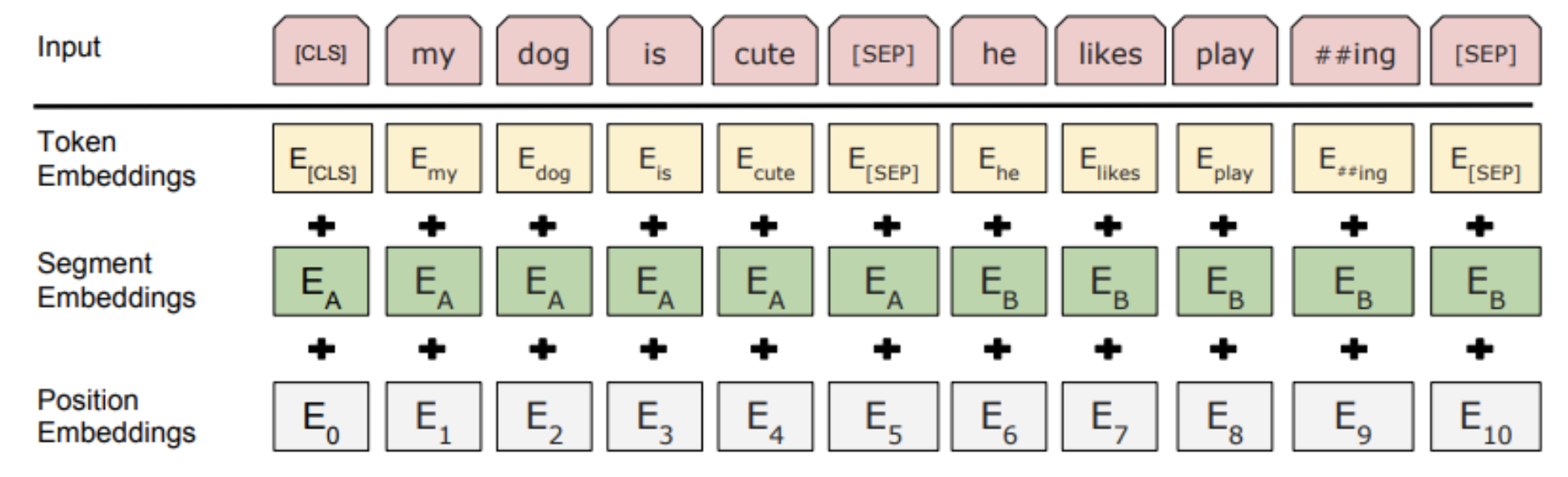
  1. 모든 categorical feature는 동일한 embedding_dims로 category feature embedding됩니다. 각 categorical feature가 고유한 임베딩 벡터를 가지게 됩니다.
  2. categorical feature인 column에 대해 column embedding이 추가됩니다. 예제 모델은 각 column을 표현할 수 있는 Embedding Layer를 추가해서 1번의 categorical feature 임베딩 벡터와 더해줍니다.
  3. 임베딩된 categorical feature는 트랜스포머에 입력됩니다. 각 트랜스포머 블럭은 multi-head self-attention layer와 feed-forward layer로 구성됩니다.
  4. categorical feature의 contextual embedding을 담당하는 마지막 Transformer layer에서 numerical feature와 concat을 수행한 뒤, MLP block에 입력됩니다.
  5. 1번 실험과 다르게 softmax classifier가 사용됩니다.(?)

논문에서 column embedding에 대한 내용을 자세하게 다루며, 모델 구조를 볼 수 있습니다.

모델 구성 순서입니다.

categorical, numerical encoding&embedding → categorical column embedding →
categorical embedding vector + column embedding vector → (Multi-head attention → skip connection →
MLP block → skip connection) → concat with numerical features → MLP block → Classifier

def create_tabtransformer_classifier(
    num_transformer_blocks,
    num_heads,
    embedding_dims,
    mlp_hidden_units_factors,
    dropout_rate,
    use_column_embedding=False,
):

    # model inputs를 생성합니다.
    inputs = create_model_inputs()
    # 각 feature를 인코딩합니다.
    encoded_categorical_feature_list, numerical_feature_list = encode_inputs(
        inputs, embedding_dims
    )
    # categorical feature는 Transformer에 입력하기 위해 stack 합니다.
    # (None, 8, 16)이 됩니다.
    encoded_categorical_features = tf.stack(encoded_categorical_feature_list, axis=1)
    # (None, 5)가 됩니다.
    numerical_features = layers.concatenate(numerical_feature_list)

    # categorical feature embedding에 column embedding을 추가합니다.
    if use_column_embedding:
        num_columns = encoded_categorical_features.shape[1]
        column_embedding = layers.Embedding(
            input_dim=num_columns, output_dim=embedding_dims
        )
        column_indices = tf.range(start=0, limit=num_columns, delta=1)
        # (None, 8, 16) + (8, 16)
        encoded_categorical_features = encoded_categorical_features + column_embedding(
            column_indices
        )

    # Create multiple layers of the Transformer block.
    for block_idx in range(num_transformer_blocks):
        # Create a multi-head attention layer.
        attention_output = layers.MultiHeadAttention(
            num_heads=num_heads,
            key_dim=embedding_dims,
            dropout=dropout_rate,
            name=f"multihead_attention_{block_idx}",
        )(encoded_categorical_features, encoded_categorical_features)
        # Skip connection 1.
        x = layers.Add(name=f"skip_connection1_{block_idx}")(
            [attention_output, encoded_categorical_features]
        )
        # Layer normalization 1.
        x = layers.LayerNormalization(name=f"layer_norm1_{block_idx}", epsilon=1e-6)(x)
        # Feedforward.
        feedforward_output = create_mlp(
            hidden_units=[embedding_dims],
            dropout_rate=dropout_rate,
            activation=keras.activations.gelu,
            normalization_layer=layers.LayerNormalization(epsilon=1e-6),
            name=f"feedforward_{block_idx}",
        )(x)
        # Skip connection 2.
        x = layers.Add(name=f"skip_connection2_{block_idx}")([feedforward_output, x])
        # Layer normalization 2.
        encoded_categorical_features = layers.LayerNormalization(
            name=f"layer_norm2_{block_idx}", epsilon=1e-6
        )(x)

    # Flatten the "contextualized" embeddings of the categorical features.
    categorical_features = layers.Flatten()(encoded_categorical_features)
    # Apply layer normalization to the numerical features.
    numerical_features = layers.LayerNormalization(epsilon=1e-6)(numerical_features)
    # Prepare the input for the final MLP block.
    features = layers.concatenate([categorical_features, numerical_features])

    # Compute MLP hidden_units.
    mlp_hidden_units = [
        factor * features.shape[-1] for factor in mlp_hidden_units_factors
    ]
    # Create final MLP.
    features = create_mlp(
        hidden_units=mlp_hidden_units,
        dropout_rate=dropout_rate,
        activation=keras.activations.selu,
        normalization_layer=layers.BatchNormalization(),
        name="MLP",
    )(features)

    # Add a sigmoid as a binary classifer.
    outputs = layers.Dense(units=1, activation="sigmoid", name="sigmoid")(features)
    model = keras.Model(inputs=inputs, outputs=outputs)
    return model


tabtransformer_model = create_tabtransformer_classifier(
    num_transformer_blocks=NUM_TRANSFORMER_BLOCKS,
    num_heads=NUM_HEADS,
    embedding_dims=EMBEDDING_DIMS,
    mlp_hidden_units_factors=MLP_HIDDEN_UNITS_FACTORS,
    dropout_rate=DROPOUT_RATE,
)

print("Total model weights:", tabtransformer_model.count_params())
keras.utils.plot_model(tabtransformer_model, show_shapes=True, rankdir="LR")

훈련 및 평가를 진행합니다.

history = run_experiment(
    model=tabtransformer_model,
    train_data_file=train_data_file,
    test_data_file=test_data_file,
    num_epochs=NUM_EPOCHS,
    learning_rate=LEARNING_RATE,
    weight_decay=WEIGHT_DECAY,
    batch_size=BATCH_SIZE,
)

추가로 아래 예제 마지막 결론을 간단히 해석해보면
TabTransformer는 Embedding이 핵심 아이디어이기 때문에 unlabeled 데이터를 pre-train에 활용할 수 있다고 합니다. 아마 semi-supervised를 표현하는 것 같아 보입니다.

TabTransformer significantly outperforms MLP and recent deep networks for tabular data while matching the performance of tree-based ensemble models. TabTransformer can be learned in end-to-end supervised training using labeled examples. For a scenario where there are a few labeled examples and a large number of unlabeled examples, a pre-training procedure can be employed to train the Transformer layers using unlabeled data. This is followed by fine-tuning of the pre-trained Transformer layers along with the top MLP layer using the labeled data.

이 글은 다음 예제를 번역한 것입니다.


Introduction

이번 예제는 CSV 파일에 포함되어 있는 구조 데이터(structured data)를 활용하여 분류 문제를 해결합니다. 데이터는 numerical과 categorical 특성들로 구성되어 있습니다. 우리는 Keras Preprocessing Layer를 사용해서 numerical 특성을 정규화하고 categorical 특성을 벡터화할 것입니다.

주의! 이번 예제는 TensorFlow 2.3 이상의 버전에서 실행해야 합니다.

The Dataset

사용할 데이터셋은 Cleveland Clinic Foundation에서 제공한 심장병 관련 데이터셋입니다. 환자 정보를 포함하고 있는 303개의 데이터(sample)로 이루어져 있으며, 각 열에서 해당 속성(feature)을 살펴볼 수 있습니다. 이를 활용하여 심장병의 여부(binary classification)를 예측해 볼 것입니다.

Age Age in years Numerical
Sex (1 = male; 0 = female) Categorical
CP Chest pain type (0, 1, 2, 3, 4) Categorical
Trestbpd Resting blood pressure (in mm Hg on admission) Numerical
Chol Serum cholesterol in mg/dl Numerical
FBS fasting blood sugar in 120 mg/dl (1 = true; 0 = false) Categorical
RestECG Resting electrocardiogram results (0, 1, 2) Categorical
Thalach Maximum heart rate achieved Numerical
Exang Exercise induced angina (1 = yes; 0 = no) Categorical
Oldpeak ST depression induced by exercise relative to rest Numerical
Slope Slope of the peak exercise ST segment Numerical
CA Number of major vessels (0-3) colored by fluoroscopy Both numerical & categorical
Thal 3 = normal; 6 = fixed defect; 7 = reversible defect Categorical
Target Diagnosis of heart disease (1 = true; 0 = false) Target


Setup

import tensorflow as tf
import numpy as np
import pandas as pd
from tensorflow import keras
from tensorflow.keras import layers

Preparing the data

데이터를 다운로드받습니다.

file_url = "http://storage.googleapis.com/download.tensorflow.org/data/heart.csv"
dataframe = pd.read_csv(file_url)

303개 데이터와 14개 column(13 feature + 1 target label)으로 이루어져 있습니다.

dataframe.shape
# (303, 14)

head() 함수로 간단히 살펴봅니다.

dataframe.head()

마지막 속성은 "target"으로 '1'이면 심장병, '0'이면 심장병이 아닌 환자를 의미합니다.

training, validation set으로 나누겠습니다.

# 20% 샘플을 뽑고,
val_dataframe = dataframe.sample(frac=0.2, random_state=1337)
# 위에서 뽑힌 샘플을 제거해서 훈련 데이터셋으로 활용합니다.
train_dataframe = dataframe.drop(val_dataframe.index)

print(
    "Using %d samples for training and %d for validation"
    % (len(train_dataframe), len(val_dataframe))
)

tf.data.Dataset 객체를 만들어줍니다.

def dataframe_to_dataset(dataframe):
    dataframe = dataframe.copy()
    labels = dataframe.pop("target")
    ds = tf.data.Dataset.from_tensor_slices((dict(dataframe), labels))
    ds = ds.shuffle(buffer_size=len(dataframe))
    
    return ds


train_ds = dataframe_to_dataset(train_dataframe)
val_ds = dataframe_to_dataset(val_dataframe)

각 Dataset은 (input, target)을 반환합니다.

  • input: dictionary of feature
  • target: 1 or 0 value
for x, y in train_ds.take(1):
    print("Input:", x)
    print("Target:", y)
    
# Input: {'age': <tf.Tensor: shape=(), dtype=int64, numpy=60>, 'sex': <tf.Tensor: shape=(), dtype=int64, numpy=1>, 'cp': <tf.Tensor: shape=(), dtype=int64, numpy=4>, 'trestbps': <tf.Tensor: shape=(), dtype=int64, numpy=117>, 'chol': <tf.Tensor: shape=(), dtype=int64, numpy=230>, 'fbs': <tf.Tensor: shape=(), dtype=int64, numpy=1>, 'restecg': <tf.Tensor: shape=(), dtype=int64, numpy=0>, 'thalach': <tf.Tensor: shape=(), dtype=int64, numpy=160>, 'exang': <tf.Tensor: shape=(), dtype=int64, numpy=1>, 'oldpeak': <tf.Tensor: shape=(), dtype=float64, numpy=1.4>, 'slope': <tf.Tensor: shape=(), dtype=int64, numpy=1>, 'ca': <tf.Tensor: shape=(), dtype=int64, numpy=2>, 'thal': <tf.Tensor: shape=(), dtype=string, numpy=b'reversible'>}
# Target: tf.Tensor(1, shape=(), dtype=int64)

Dataset에 배치 크기를 설정합니다.

train_ds = train_ds.batch(32)
val_ds = val_ds.batch(32)


Feature preprocessing with Keras layers

정수형태로 인코딩되어 있는 categorical feature은 다음과 같습니다.

  • sex, cp, fbs, restecg, exang, ca

CategoryEncoding() layer를 사용해서 one-hot encoding 형태로 바꿔줄 것입니다. 또, thal은 문자형태로 인코딩되어 있는 categorical feature입니다. 먼저 StringLookup() layer를 사용해서 해당 속성이 가지고 있는 값들을 전부 index 형태로 변환하고, CategoryEncoding() layer를 사용해서 one-hot 인코딩을 동일하게 진행해줄 것입니다.

마지막으로, 연속적인 정수 형태인 feature는 다음과 같습니다.

  • age, trestbps, chol, thalach, oldpeak, slope

이들에게는 Normalization() layer를 사용해서 평균 0, 표준 편차를 1로 만들어 줄 것입니다.

이 작업을 수행하기 위해 세 가지 유틸리티 함수를 정의해서 사용합니다.

  • encode_numerical_feature: Normalization을 적용하기 위한 함수
  • encode_string_categorical_feature: 문자 형태로 된 열에 대해 one-hot encoding을 적용
  • encode_integer_categorical_feature: 숫자 형태로 된 열에 대해 one-hot encoding을 적용
from tensorflow.keras.layers.experimental.preprocessing import Normalization
from tensorflow.keras.layers.experimental.preprocessing import CategoryEncoding
from tensorflow.keras.layers.experimental.preprocessing import StringLookup


def encode_numerical_feature(feature, name, dataset):
    # Normalization layer 정의
    normalizer = Normalization()

    # 적용할 열만 가져옵니다.
    feature_ds = dataset.map(lambda x, y: x[name])
    feature_ds = feature_ds.map(lambda x: tf.expand_dims(x, -1))

    # 데이터의 통계치 학습
    normalizer.adapt(feature_ds)

    # 정규화 진행
    encoded_feature = normalizer(feature)
    
    return encoded_feature


def encode_string_categorical_feature(feature, name, dataset):
    # 문자열로 되어 있는 값을 integer 형태로 변환하기 위한 StringLookup() 함수 정의
    index = StringLookup()
    # one-hot encoding 진행을 위한 함수 정의
    encoder = CategoryEncoding(output_mode="binary")
    
    # 적용할 열만 가져옵니다.
    feature_ds = dataset.map(lambda x, y: x[name])
    feature_ds = feature_ds.map(lambda x: tf.expand_dims(x, -1))
    
    # 전체 순서: index adapt -> index 형태로 변환 -> categorical encoding adapt -> categorical 형태로 변환
    
    # feature_ds가 반환하는 문자열 데이터가 어떤 것이 있는지 확인합니다.
    # 문자열로 된 값과, integer index를 부여하기 위한 작업입니다.
    index.adapt(feature_ds)

    # (실제 반환 데이터) integer 형태로 변환합니다.
    encoded_feature = index(feature)
    
    # Dataset 객체가 index 변환 작업을 수행하도록 적용해줍니다.
    feature_ds = feature_ds.map(index)
    
    # feature_ds가 반환하는 index 데이터가 어떤 것이 있는지 확인합니다.
    encoder.adapt(feature_ds)

    # (실제 반환 데이터) one-hot encoding을 적용하고 return합니다.
    # 데이터셋 객체에 다시 map 해줄 필요는 없습니다.
    encoded_feature = encoder(encoded_feature)
    
    return encoded_feature

# 위와 동일
def encode_integer_categorical_feature(feature, name, dataset):
    # Create a CategoryEncoding for our integer indices
    encoder = CategoryEncoding(output_mode="binary")

    # Prepare a Dataset that only yields our feature
    feature_ds = dataset.map(lambda x, y: x[name])
    feature_ds = feature_ds.map(lambda x: tf.expand_dims(x, -1))

    # Learn the space of possible indices
    encoder.adapt(feature_ds)

    # Apply one-hot encoding to our indices
    encoded_feature = encoder(feature)
    return encoded_feature


Build a model

end-to-end 모델을 만들어봅니다.

# Numerical -> one-hot encoding
sex = keras.Input(shape=(1,), name="sex", dtype="int64")
cp = keras.Input(shape=(1,), name="cp", dtype="int64")
fbs = keras.Input(shape=(1,), name="fbs", dtype="int64")
restecg = keras.Input(shape=(1,), name="restecg", dtype="int64")
exang = keras.Input(shape=(1,), name="exang", dtype="int64")
ca = keras.Input(shape=(1,), name="ca", dtype="int64")

# String -> one-hot encoding
thal = keras.Input(shape=(1,), name="thal", dtype="string")

# Numerical features
age = keras.Input(shape=(1,), name="age")
trestbps = keras.Input(shape=(1,), name="trestbps")
chol = keras.Input(shape=(1,), name="chol")
thalach = keras.Input(shape=(1,), name="thalach")
oldpeak = keras.Input(shape=(1,), name="oldpeak")
slope = keras.Input(shape=(1,), name="slope")

all_inputs = [sex, cp, fbs,
                restecg, exang, ca,
                thal, age, trestbps,
                chol, thalach, oldpeak,slope]

# Integer categorical features
sex_encoded = encode_integer_categorical_feature(sex, "sex", train_ds)
cp_encoded = encode_integer_categorical_feature(cp, "cp", train_ds)
fbs_encoded = encode_integer_categorical_feature(fbs, "fbs", train_ds)
restecg_encoded = encode_integer_categorical_feature(restecg, "restecg", train_ds)
exang_encoded = encode_integer_categorical_feature(exang, "exang", train_ds)
ca_encoded = encode_integer_categorical_feature(ca, "ca", train_ds)

# String categorical features
thal_encoded = encode_string_categorical_feature(thal, "thal", train_ds)

# Numerical features
age_encoded = encode_numerical_feature(age, "age", train_ds)
trestbps_encoded = encode_numerical_feature(trestbps, "trestbps", train_ds)
chol_encoded = encode_numerical_feature(chol, "chol", train_ds)
thalach_encoded = encode_numerical_feature(thalach, "thalach", train_ds)
oldpeak_encoded = encode_numerical_feature(oldpeak, "oldpeak", train_ds)
slope_encoded = encode_numerical_feature(slope, "slope", train_ds)

all_features = layers.concatenate(
    [
        sex_encoded,
        cp_encoded,
        fbs_encoded,
        restecg_encoded,
        exang_encoded,
        slope_encoded,
        ca_encoded,
        thal_encoded,
        age_encoded,
        trestbps_encoded,
        chol_encoded,
        thalach_encoded,
        oldpeak_encoded,
    ]
)

x = layers.Dense(32, activation="relu")(all_features)
x = layers.Dropout(0.5)(x)

output = layers.Dense(1, activation="sigmoid")(x)

# 모델 생성
model = keras.Model(all_inputs, output)
model.compile("adam", "binary_crossentropy", metrics=["accuracy"])


Train the model

model.fit(train_ds, epochs=50, validation_data=val_ds)

약 82% 정확도를 얻을 수 있었습니다.

Inference on new data

model.predict()를 활용해서 새로운 환자의 심장병 여부를 확인해보죠.

  1. batch dimension을 까먹지 않도록 주의해야 합니다. 모델은 batch_dimension에서 과정에 수행됩니다.
  2. 새로운 샘플에서 값을 tensor 형태로 변환하기 위해 convert_to_tensor 활용
sample = {
    "age": 60,
    "sex": 1,
    "cp": 1,
    "trestbps": 145,
    "chol": 233,
    "fbs": 1,
    "restecg": 2,
    "thalach": 150,
    "exang": 0,
    "oldpeak": 2.3,
    "slope": 3,
    "ca": 0,
    "thal": "fixed",
}

input_dict = {name: tf.convert_to_tensor([value]) for name, value in sample.items()}
predictions = model.predict(input_dict)

print(
    "This particular patient had a %.1f percent probability "
    "of having a heart disease, as evaluated by our model." % (100 * predictions[0][0],)
)

# This particular patient had a 20.8 percent probability of having a heart disease, 
# as evaluated by our model.


이 글은 다음 예제를 번역한 것입니다.


Introduction

이 예제는 JPEG 파일을 직접 저장하고, 미리 학습된 모델을 사용하지 않으면서 이미지 분류를 어떻게 행하는지 알아보는 예제입니다. 'Cats vs Dogs' 데이터셋을 케라스를 활용하여 분류해봅니다.

데이터셋 생성을 위해 image_dataset_from_directory를 사용하고, 표준화와 augmentation을 위해 Keras Preprocessing Layer를 사용해봅니다.

Setup

import tensorflow as tf
from tensorflow import keras
from tensorflow.keras import layers


Load the data: the Cats vs Dogs dataset

Raw data download

먼저, 765M 크기의 데이터를 다운로드합니다.
예제와 다르게 그냥 쥬피터 노트북 상에서 zip파일을 다운받고 싶으면, 아래 코드를 활용하면 됩니다.

import requests

target_path = 'datasets.zip'

url = 'https://download.microsoft.com/download/3/E/1/3E1C3F21-ECDB-4869-8368-6DEBA77B919F/kagglecatsanddogs_3367a.zip'
response = requests.get(url, stream = True)
handle = open(target_path, 'wb')

for chunk in response.iter_content(chunk_size = 512):
    if chunk:
        handle.write(chunk)
        
handle.close()   

압축을 풀었다면, 최상위 폴더에는 Cat, Dog 하위 폴더가 존재합니다.

Filter out corrupted images

손상된 이미지는 어디에나 존재합니다. 여기서는 "JFIF" 헤더를 가진 이미지를 필터링해보겠습니다.
필터링 시, 해당 헤더가 아니면 손상된 이미지이므로 제거합니다.

import os

num_skipped = 0
for folder_name in ("Cat", "Dog"):
    folder_path = os.path.join("PetImages", folder_name)
    for fname in os.listdir(folder_path):
        fpath = os.path.join(folder_path, fname) # PetImages/Cat/63.jpg
        try:
            fobj = open(fpath, "rb")
            # fobj.peek(10)은 10바이트를 가져오는데, 여기서는 보통
            # 헤더를 읽기 위해 전체를 가져온다고 생각해도 무방합니다.
            is_jfif = tf.compat.as_bytes("JFIF") in fobj.peek(10)
        finally:
            fobj.close()

        if not is_jfif:
            num_skipped += 1
            # Delete corrupted image
            os.remove(fpath)

print("Deleted %d images" % num_skipped)


Generate a Dataset

image_size = (180, 180)
batch_size = 32

train_ds = tf.keras.preprocessing.image_dataset_from_directory(
    "PetImages",
    validation_split=0.2,
    subset="training",
    seed=1337,
    image_size=image_size,
    batch_size=batch_size,
)
val_ds = tf.keras.preprocessing.image_dataset_from_directory(
    "PetImages",
    validation_split=0.2,
    subset="validation",
    seed=1337,
    image_size=image_size,
    batch_size=batch_size,
)

Visualize the data

9개 이미지를 그려봅니다. '1'은 Dog이고, '0'은 Cat에 해당합니다.

import matplotlib.pyplot as plt

# figure 크기를 조절합니다.
plt.figure(figsize=(10, 10))

# 배치 하나를 가져옵니다.
for images, labels in train_ds.take(1):
    for i in range(9):
        ax = plt.subplot(3, 3, i + 1)
        plt.imshow(images[i].numpy().astype("uint8"))
        plt.title(int(labels[i]))
        plt.axis("off")

Using Image data augmentation

데이터가 다양하지 않거나, 데이터 개수가 충분하지 않을때 랜덤으로 회전시키거나 fliping하는 등 augmentation을 활용하면 이를 해결할 수 있습니다. 이는 모델이 다양한 데이터를 볼 수 있게 도와줌과 동시에 이를 통해 Overfitting을 (어느정도) 극복할 수 있습니다.

data_augmentation = keras.Sequential(
    [
        layers.experimental.preprocessing.RandomFlip("horizontal"),
        layers.experimental.preprocessing.RandomRotation(0.1),
    ]
)

data_augmentation을 통해 변형된 이미지를 그려봅니다.

plt.figure(figsize=(10, 10))
for images, _ in train_ds.take(1):
    for i in range(9):
        augmented_images = data_augmentation(images)
        ax = plt.subplot(3, 3, i + 1)
        plt.imshow(augmented_images[0].numpy().astype("uint8"))
        plt.axis("off")


Standardizing the data

현재 우리가 사용할 이미지는 픽셀 type float32, 크기는 180x180으로 이미 어느정도 표준화가 되어 있습니다. 하지만 RGB channel의 값들이 [0, 255] 값을 가지고 있어, 신경망을 사용하기엔 적합하지 않습니다. 따라서 Rescaling layer를 활용해서 [0, 1] 범위로 변환해줄 것입니다.


Two options to preprocess the data

augmentation을 적용할 수 있는 두 가지 방법이 있습니다.

>> Option 1: Make it part of the model like this:

inputs = keras.Input(shape=input_shape)
x = data_augmentation(inputs)
x = layers.experimental.preprocessing.Rescaling(1./255)(x)
...  # Rest of the model

이 방법은 모델 실행에서 동시에 사용될 수 있기 때문에 GPU를 사용한다는 큰 장점을 활용할 수 있습니다.

이 방법은 test time에는 동작하지 않기 때문에, evaluate(), predict()에서는 활용되지 않고, 오로지 fit() 동안에만 사용됩니다. 또한, GPU를 보유하고 있다면 이 방법을 긍정적으로 고려해볼 수 있습니다.

>> Option 2: apply it to the dataset, so as to obtain a dataset that yields batches of augmented images, like this:

augmented_train_ds = train_ds.map(
  lambda x, y: (data_augmentation(x, training=True), y))

이 방법은 CPU에서 주로 사용되고, 버퍼를 통해 모델에 입력됩니다.

CPU를 활용하여 학습하는 경우라면 이 방법이 더 효과적입니다.


Configure the dataset for performance

prefetch 옵션을 활용하면 더욱 효율적으로 데이터를 생성하여 모델에 입력할 수 있습니다.

train_ds = train_ds.prefetch(buffer_size=32)
val_ds = val_ds.prefetch(buffer_size=32)


Build a model

Xception의 small version을 작성해보겠습니다. 이 모델에 대해서는 최적화를 진행하지 않을 것이고, 만약 최적화에 관심이 있다면 Keras Tuner를 고려해보세요.

강조 사항:

  • data_augmentation을 사용하고, 추가로 Rescaling layer를 활용합니다.
  • 마지막 classification layer에 Dropout을 추가합니다.
def make_model(input_shape, num_classes):
    inputs = keras.Input(shape=input_shape)
    # 본격적으로 모델에 입력하기 전에 여기서 augmentation이 진행됩니다.
    # inference time에는 동작하지 않습니다.
    x = data_augmentation(inputs)

    # [0, 1] 변환을 위해 Rescaling Layer를 활용합니다.
    x = layers.experimental.preprocessing.Rescaling(1.0 / 255)(x)
    x = layers.Conv2D(32, 3, strides=2, padding="same")(x)
    x = layers.BatchNormalization()(x)
    x = layers.Activation("relu")(x)

    x = layers.Conv2D(64, 3, padding="same")(x)
    x = layers.BatchNormalization()(x)
    x = layers.Activation("relu")(x)

    previous_block_activation = x  # Set aside residual

    for size in [128, 256, 512, 728]:
        x = layers.Activation("relu")(x)
        x = layers.SeparableConv2D(size, 3, padding="same")(x)
        x = layers.BatchNormalization()(x)

        x = layers.Activation("relu")(x)
        x = layers.SeparableConv2D(size, 3, padding="same")(x)
        x = layers.BatchNormalization()(x)

        x = layers.MaxPooling2D(3, strides=2, padding="same")(x)

        # Project residual
        residual = layers.Conv2D(size, 1, strides=2, padding="same")(
            previous_block_activation)
        x = layers.add([x, residual])  # Add back residual
        previous_block_activation = x  # Set aside next residual

    x = layers.SeparableConv2D(1024, 3, padding="same")(x)
    x = layers.BatchNormalization()(x)
    x = layers.Activation("relu")(x)

    x = layers.GlobalAveragePooling2D()(x)
    if num_classes == 2:
        activation = "sigmoid"
        units = 1
    else:
        activation = "softmax"
        units = num_classes

    x = layers.Dropout(0.5)(x)
    outputs = layers.Dense(units, activation=activation)(x)
    
    return keras.Model(inputs, outputs)

# image size에 (3, ) 채널을 추가합니다.
model = make_model(input_shape=image_size + (3,), num_classes=2)


Train the model

epochs = 50

callbacks = [
    keras.callbacks.ModelCheckpoint("save_at_{epoch}.h5"),
]
model.compile(optimizer=keras.optimizers.Adam(1e-3),
              loss="binary_crossentropy",
              metrics=["accuracy"])
model.fit(train_ds, epochs=epochs, 
          callbacks=callbacks, validation_data=val_ds)

학습을 진행해보세요.


Run inference on new data

inference time에는 Dropout과 data augmentation이 비활성화 상태가 됩니다.
하지만 Rescaling layer는 그대로 활용되기 때문에 테스트용 데이터로 추론을 진행할 때 올바른 결과를 얻을 수 있습니다.

img = keras.preprocessing.image.load_img("PetImages/Cat/6779.jpg", 
                                         target_size=image_size)
img_array = keras.preprocessing.image.img_to_array(img)
img_array = tf.expand_dims(img_array, 0)  # Create batch axis

predictions = model.predict(img_array)
score = predictions[0]
print(
    "This image is %.2f percent cat and %.2f percent dog."
    % (100 * (1 - score), 100 * score)
)

예전에 Pytorch의 Image augmentation 방법을 보고 커스텀이 되게 편리하게 구성된 것 같아 TensorFlow도 이와 같은 방법으로 augmentation하도록 만들어줬으면 좋겠다는 생각을 하고 있었는데, 연동 가능한 라이브러리 albumentation이 있었습니다.
(만들어진지 좀 됬는데 늦게 알게 됨..)

transforms.Compose([
	transforms.CenterCrop(10),
	transforms.ToTensor(),
])

torchvision의 augmentation 방법

사실 아래 공식 홈페이지 튜토리얼 코드를 보면 TensorFlow도 이와 같은 방법으로 Keras Layer를 활용한 augmentation이 가능토록 제공하고 있고, 앞으로도 이러한 방법으로 제공할 예정인가 싶습니다.

data_augmentation = tf.keras.Sequential([
  layers.experimental.preprocessing.RandomFlip("horizontal_and_vertical"),
  layers.experimental.preprocessing.RandomRotation(0.2),
])

출처: www.tensorflow.org/tutorials/images/data_augmentation?hl=ko


tf.image를 사용하는 방법

albumentation 라이브러리를 사용해보기 전에, tf.image를 사용해서 어떻게 augmentation 할 수 있는지 코드를 첨부합니다.

test = tf.data.Dataset.from_tensor_slices(dict(df))

# 이미지와 레이블을 얻습니다.
def get_image_label(dt):
    img_path = dt['image']
    
    image = tf.io.read_file(img_path)
    image = tf.image.decode_jpeg(image)
    image = tf.image.convert_image_dtype(image, tf.float32)
    image = tf.image.resize(image, [IMG_SIZE, IMG_SIZE])
    image = (image / 255.0)

    label = []
    
    for key in class_col:
        label.append(dt[key])
    
    return image, label

# data augment
# refer: https://www.tensorflow.org/tutorials/images/data_augmentation
def augment(image,label):
    # Add 6 pixels of padding
    image = tf.image.resize_with_crop_or_pad(image, IMG_SIZE + 6, IMG_SIZE + 6) 
    # Random crop back to the original size
    image = tf.image.random_crop(image, size=[IMG_SIZE, IMG_SIZE, 3])
    image = tf.image.random_brightness(image, max_delta=0.5) # Random brightness
    image = tf.clip_by_value(image, 0, 1)

    return image, label

    
dataset = test.map(get_image_label)
dataset = dataset.shuffle(50).map(augment).batch(4)

이 방법도 괜찮긴하지만 문제는 tf.Dataset 작동 구조를 알아야 정확히 쓸 수 있습니다.
map 함수 작동 방식이라던가, shuffle과 batch의 위치 등등..

확실히 위 방법보다 augmentation 방법을 Layer 구조로 가져가는게 훨씬 가독성이 좋아보이기도 합니다. 아래처럼요.

model = tf.keras.Sequential([
  resize_and_rescale,
  data_augmentation,
  layers.Conv2D(16, 3, padding='same', activation='relu'),
  layers.MaxPooling2D(),
  # Rest of your model
])

resize_and_rescale과 data_augmentation을 Sequential 안에 Layer 형태로 사용하고 있습니다.

하지만 아직 많이 쓰이고 있는 방법은 아닌 것 같기에 확실하게 자리잡기 전(?)까지 다른 방법을 사용해도 꽤나 무방합니다.


Albumentation 라이브러리를 사용하는 방법

사용하는 방법은 꽤나 단순합니다. 위에서 예제로 보여드렸던 코드와 형식이 동일하니까요.

먼저, 필요 라이브러리를 불러옵니다.

from tensorflow.keras.datasets import cifar10

import albumentations
import cv2
import numpy as np
import matplotlib.pyplot as plt
import cv2
# augmentation method를 import합니다.
from albumentations import (
    Compose, HorizontalFlip, CLAHE, HueSaturationValue,
    RandomBrightness, RandomContrast, RandomGamma,
    ToFloat, ShiftScaleRotate
)

torchvision의 Compose, TensorFlow의 Sequential과 Albumentation의 Compose의 사용되는 장소가 같습니다. 위에서 호출한 함수 외에도 다양한 augmentation 방법을 제공합니다. 더 궁금하면 공식 문서를 참조하고, 자세히 설명되어 있습니다.

albumentations.ai/docs/getting_started/image_augmentation/

이제 다양한 함수를 Compose안에 list 형태로 제공하고, 사용할 준비를 끝마칩니다.

# 각 함수에 대한 설명은
# https://albumentations.ai/docs/
# document를 참고하세요.
Aug_train = Compose([
    HorizontalFlip(p=0.5),
    RandomContrast(limit=0.2, p=0.5),
    RandomGamma(gamma_limit=(80, 120), p=0.5),
    RandomBrightness(limit=0.2, p=0.5),
    HueSaturationValue(hue_shift_limit=5, sat_shift_limit=20,
                       val_shift_limit=10, p=.9),
    ShiftScaleRotate(
        shift_limit=0.0625, scale_limit=0.1, 
        rotate_limit=15, border_mode=cv2.BORDER_REFLECT_101, p=0.8), 
    ToFloat(max_value=255)
])

Aug_test = Compose([
    ToFloat(max_value=255)
])


실험하기에 가장 좋은 예제는 tensorflow.keras.datasets에서 제공하는 CIFAR-10입니다.
또, Sequence 클래스를 상속받아 제네레이터처럼 활용할 수 있도록 합니다.
아래 코드 __getitem__ 부분의 self.augment(image=x)["image"]에서 변환 작업이 수행됩니다.

from tensorflow.python.keras.utils.data_utils import Sequence

# Sequence 클래스를 상속받아 generator 형태로 사용합니다.
class CIFAR10Dataset(Sequence):
    def __init__(self, x_set, y_set, batch_size, augmentations):
        self.x, self.y = x_set, y_set
        self.batch_size = batch_size
        self.augment = augmentations

    def __len__(self):
        return int(np.ceil(len(self.x) / float(self.batch_size)))

    # 지정 배치 크기만큼 데이터를 로드합니다.
    def __getitem__(self, idx):
        batch_x = self.x[idx * self.batch_size:(idx + 1) * self.batch_size]
        batch_y = self.y[idx * self.batch_size:(idx + 1) * self.batch_size]
        
        # augmentation을 적용해서 numpy array에 stack합니다.
        return np.stack([
            self.augment(image=x)["image"] for x in batch_x
        ], axis=0), np.array(batch_y)

# CIFAR-10 Dataset을 불러옵니다.
(x_train, y_train), (x_test, y_test) = cifar10.load_data()

BATCH_SIZE = 8

# Dataset을 생성합니다.
train_gen = CIFAR10Dataset(x_train, y_train, BATCH_SIZE, Aug_train)
test_gen = CIFAR10Dataset(x_test, y_test, BATCH_SIZE, Aug_test)

train_gen을 통해 이미지를 그려보면 다음과 같이 변환이 일어난 것을 볼 수 있습니다.

# 데이터를 그려봅시다.
images, labels = next(iter(train_gen))

fig = plt.figure()

for i, (image, label) in enumerate(zip(images, labels)):
    ax = fig.add_subplot(3, 3, i + 1)
    ax.imshow(image)
    ax.set_xlabel(label)
    ax.set_xticks([]); ax.set_yticks([])

plt.tight_layout()
plt.show()

Augmentation이 수행된 이미지


Reference

텐서플로우 공식 홈페이지

Albumentation Document

medium.com/the-artificial-impostor/custom-image-augmentation-with-keras-70595b01aeac

다양한 문제를 해결하고, 만들어내고 있는 GPT-3가 연일 화제가 되면서 인공지능 관련 모든 분야에서 굉장히 뜨거운 반응을 보이고 있습니다. NLP뿐만 아니라 Computer Vision task도 해결할 수 있음을 보였는데, 이러한 결과가 매우 매력적일 수밖에 없습니다. 물론 사용된 파라미터 수, 학습 시간 등을 고려해보면 개인적으로 어떻게 활용할 수 있을까에 대한 좌절감도 동시에 다가옵니다.

트렌드를 빠른 속도로 파악하고 제시하고 있는 Andrew Ng님도 Transformer, BERT, GPT-3가 매우 대단한 결과를 보이고 있음을 이야기하고, NLP 분야의 수요가 지속적으로 늘어날 것을 이야기할 정도입니다.

BERT에 관심이 있는, NLP에 관심이 있다면 반드시 밑의 세 가지 논문을 요약으로라도 읽어봐야 합니다.

이 중에서도 이번 글에서는 BERT를 직접 공부하면서 도움이 될만한 몇 가지 사항을 정리하였습니다. 이전에 연관 논문을 읽고 BERT라는 주제를 공부하면 매우 도움이 되겠지만, 순서가 뒤바뀌어도 문제 될게 없습니다.


BERT

Transformer architecture을 중점적으로 사용한 BERT는 Bidirectional Encoder Representations from Transformers을 의미합니다. 바로 BERT에서 살펴볼 주요한 사항을 살펴보겠습니다.

들어가기 전에, BERT는 text classification, answering 등을 해결할 수 있는 모델이지만, 이보다는 Language Representation을 해결하기 위해 고안된 구조라는 것을 알아주세요.
(즉, 단어, 문장, 언어를 어떻게 표현할까에 관한 고민이고, 이를 잘 표현할 수 있다면 다양한 task를 해결할 수 있습니다.)


BERT는 양방향성을 포함하여 문맥을 더욱 자연스럽게 파악할 수 있습니다.

Bidirectional은 직역하는 것과 동일하게 BERT 모델이 양방향성 특성을 가지고 이를 적용할 수 있다는 것을 의미합니다.
이를 사용하기 이전의 대부분 모델은 문장이 존재하면 왼쪽에서 오른쪽으로 진행하여 문맥(context)를 파악하는 방법을 지녔는데요. 이는 전체 문장을 파악하는 데 있어서 당연히 제한될 수 밖에 없는 한계점입니다.

쉽게 생각해보면, '나는 하늘이 예쁘다고 생각한다'라는 문장을 이해할 때, 단순히 '하늘'이라는 명사를 정해놓고 '예쁘다'라는 표현을 사용하지는 않습니다. '예쁘다'를 표현하고 싶어서 '하늘'이라는 명사를 선택했을 수도 있습니다. 즉, 앞에서 뒤를 볼수도 있지만, 뒤에서 앞을 보는 경우도 충분히 이해할 수 있어야 전체 맥락을 완전히 파악할 수 있다는 것이죠.

단방향성, 양방향성

이 예가 아니더라도 동의어를 파악하기 위해선 앞뒤 단어의 관계성을 파악해야 한다는 점을 이해할 수 있습니다.

-> 긍정적인 의미의 잘했다와 부정적인 의미의 잘했다.
ex1) A: "나 오늘 주식 올랐어!", B: "진짜 잘했다"
ex2) A: "나 오늘 주식으로 망했어", B: "진짜 잘~했다"

결론적으로는 기존 단방향성 모델은 성능 향상, 문맥 파악에 한계점이 존재했었고, 이를 해결하기 위해 양방향성을 띄는 모델을 제안하는 방향으로 진행된 것입니다. (RNN과 Bidirectional RNN의 차이점을 살펴도 같은 문제를 해결하기 위한 것을 알 수 있습니다)


BERT는 pre-training이 가능한 모델입니다.

이전에 존재하던 NLP 모델은 pre-training이 어려웠기 때문에 특정 task가 존재할 경우 처음부터 학습시켜야 하는 단점이 존재했습니다. 각종 Image task를 해결하는 데 있어서도 pre-trianing이 매우 큰 역할을 하고 있다는 점을 보면, NLP에서도 여러 task에 transfer하기 위해서는 이를 활용할 수 있는 모델이 매우 시급했습니다.

이에 대한 연구가 매우 활발히 진행되었고, 대표적으로 ELMO, XLNet, BERT, GPT 등 모델이 만들어지게 되었죠.

엄청난 수의 Wikipedia와 BooksCorpus 단어를 학습한 BERT를 다양한 task에 적용하고, fine-tuning해서 사용할 수 있는 것은 매우 큰 장점으로 우리에게 다가올 수 밖에 없습니다.


BERT는 주로 어떤 문제에 적용할 수 있을까요?

대표적으로 해결할 수 있는 몇 가지 문제를 알려드리겠습니다. 하지만 여기서 설명되지 않은 다양한 분야가 매우 다양하게 존재하다는 것을 잊어버리면 안됩니다. 아래 문제들은 대부분 NLP task에서 볼 수 있는 대표적인 문제들입니다.

  1. Question and Answering
    - 주어진 질문에 적합하게 대답해야하는 매우 대표적인 문제입니다.
    - KoSQuAD, Visual QA etc.
  2. Machine Translation
    - 구글 번역기, 네이버 파파고입니다.
  3. 문장 주제 찾기 또는 분류하기
    - 역시나 기존 NLP에서도 해결할 수 있는 문제는 당연히 해결할 수 있습니다.
  4. 사람처럼 대화하기
    - 이와 같은 주제에선 매우 강력함을 보여줍니다.
  5. 이외에도 직접 정의한 다양한 문제에도 적용 가능합니다. 물론 꼭 NLP task일 필요는 없습니다.


어떻게 학습되었는지 알아보자

기본적으로 BERT는 'Attention is all you need" 논문에서 볼 수 있는 Transformer 구조를 중점적으로 사용한 구조입니다. 특히
self-attiotion layer를 여러 개 사용하여 문장에 포함되어 있는 token 사이의 의미 관계를 잘 추출할 수 있습니다.

BERT는 transformer 구조를 사용하면서도 encoder 부분만 사용(아래 그림에서 왼쪽 부분)하여 학습을 진행했는데요. 기존 모델은 대부분 encoder-decoder으로 이루어져 있으며, GPT 또한, decoder 부분을 사용하여 text generation 문제를 해결하는 모델입니다. Transformer 구조 역시, input에서 text의 표현을 학습하고, decoder에서 우리가 원하는 task의 결과물을 만드는 방식으로 학습이 진행됩니다.

Attention mechanism - Attention Paper

BERT는 decoder를 사용하지 않고, 두 가지 대표적인 학습 방법으로 encoder를 학습시킨 후에 특정 task의 fine-tuning을 활용하여 결과물을 얻는 방법으로 사용됩니다.


어떻게 학습되었는지 알아보자 - input Representation

역시나 어떤 주제이던 데이터 처리에 관한 이야기는 빠질 수가 없습니다. BERT는 학습을 위해 기존 transformer의 input 구조를 사용하면서도 추가로 변형하여 사용합니다. Tokenization은 WorldPiece 방법을 사용하고 있습니다.

Input Representation - BERT paper

위 그림처럼 세 가지 임베딩(Token, Segment, Position)을 사용해서 문장을 표현합니다.

먼저 Token Embedding에서는 두 가지 특수 토큰(CLS, SEP)을 사용하여 문장을 구별하게 되는데요. Special Classification token(CLS)은 모든 문장의 가장 첫 번째(문장의 시작) 토큰으로 삽입됩니다. 이 토큰은 Classification task에서는 사용되지만, 그렇지 않을 경우엔 무시됩니다. 
또, Special Separator token(SEP)을 사용하여 첫 번째 문장과 두 번째 문장을 구별합니다. 여기에 segment Embedding을 더해서 앞뒤 문장을 더욱 쉽게 구별할 수 있도록 도와줍니다. 이 토큰은 각 문장의 끝에 삽입됩니다.

Position Embedding은 transformer 구조에서도 사용된 방법으로 그림고 같이 각 토큰의 위치를 알려주는 임베딩입니다.
최종적으로 세 가지 임베딩을 더한 임베딩을 input으로 사용하게 됩니다.


어떻게 학습되었는지 알아보자 - Pre-training

 BERT는 문장 표현을 학습하기 위해 두 가지 unsupervised 방법을 사용합니다.

  1. Masked Language Model
  2. Next Sentence Model


Masked Language Model (MLM)

문장에서 단어 중의 일부를 [Mask] 토큰으로 바꾼 뒤, 가려진 단어를 예측하도록 학습합니다. 이 과정에서 BERT는 문맥을 파악하는 능력을 기르게 됩니다.

ex) 나는 하늘이 예쁘다고 생각한다 -> 나는 하늘이 [Mask] 생각한다.
ex) 나는 하늘이 예쁘다고 생각한다 -> 나는 하늘이 흐리다고 생각한다.
ex) 나는 하늘이 예쁘다고 생각한다 -> 나는 하늘이 예쁘다고 생각한다.

추가적으로 더욱 다양한 표현을 학습할 수 있도록 80%는 [Mask] 토큰으로 바꾸어 학습하지만, 나머지 10%는 token을 random word로 바꾸고, 마지막 10%는 원본 word 그대로를 사용하게 됩니다.

Next Sentence Prediction (NSP)

다음 문장이 올바른 문장인지 맞추는 문제입니다. 이 문제를 통해 두 문장 사이의 관계를 학습하게 됩니다. 

문장 A와 B를 이어 붙이는데, B는 50% 확률로 관련 있는 문장(IsNext label) 또는 관련 없는 문장(NotNext label)을 사용합니다.
QA(Question Answering)나 NLI(Natural Language Inference) task의 성능 향상에 영향을 끼친다고 합니다.


이런 방식으로 학습된 BERT를 fine-tuning할 때는 (Classification task라면)Image task에서의 fine-tuning과 비슷하게 class label 개수만큼의 output을 가지는 Dense Layer를 붙여서 사용합니다.


Reference