Dataset.map(f)는 입력 데이터셋의 각 원소에 주어진 함수 f를 적용하여 새로운 데이터셋을 생성해줍니다. 함수형 프로그래밍 언어에서 리스트 또는 기타 구조에 적용되는 map() 함수를 기반으로 합니다. 함수 f는 입력에서 단일 요소인 tf.Tensor 오브젝트를 받으며, 새로운 데이터셋에 포함될 tf.Tensor 오브젝트를 반환합니다. 이에 대한 구현은 TensorFlow 연산을 사용하여 한 요소를 다른 요소로 변환합니다.
이번 절에서는 Dataset.map()의 사용 방법을 다룹니다.
Decoding image data and resizing it
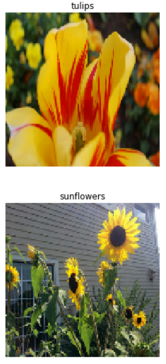
실제 환경의 이미지 데이터를 학습시킬 때, 보통 서로 다른 크기의 이미지를 공통 크기로 변환하여 고정 크기의 배치를 사용합니다. flower 데이터셋을 사용해봅시다.
# Reads an image from a file, decodes it into a dense tensor, and resizes it
# to a fixed shape.
def parse_image(filename):
  parts = tf.strings.split(filename, '/')
  label = parts[-2]

  image = tf.io.read_file(filename)
  image = tf.image.decode_jpeg(image)
  image = tf.image.convert_image_dtype(image, tf.float32)
  image = tf.image.resize(image, [128, 128])
  return image, label
images_ds = list_ds.map(parse_image)

for image, label in images_ds.take(2):
  show(image, label)
Applying arbitrary Python logic
데이터 전처리 작업에 TensorFlow 연산을 사용하면 성능적으로 이득을 볼 수 있습니다. 하지만 가끔은 입력 데이터를 처리하기 위해 파이썬 라이브러리 함수가 유용할 때가 있습니다. 이를 위해 Dataset.map()에서 tf.py_function()을 사용하세요.
예를 들어, random rotation 처리를 적용하고 싶지만 TensorFlow 연산은 tf.image의 tf.image.rot90 함수만 제공하기 때문에 유용하지 않을 수 있습니다. tf.py_function()을 경험해보기 위해, scipy.ndimage.rotate 함수를 사용해보죠.
또는, dense한 prediction을 원할 경우, feature와 label을 한 단계씩 이동(shift)할 수 있습니다.
def dense_1_step(batch):
  # Shift features and labels one step relative to each other.
  return batch[:-1], batch[1:]

predict_dense_1_step = batches.map(dense_1_step)

for features, label in predict_dense_1_step.take(3):
  print(features.numpy(), " => ", label.numpy())
batches = range_ds.batch(15, drop_remainder=True)

def label_next_5_steps(batch):
  return (batch[:-5],   # Take the first 5 steps
          batch[-5:])   # take the remainder

predict_5_steps = batches.map(label_next_5_steps)

for features, label in predict_5_steps.take(3):
  print(features.numpy(), " => ", label.numpy())
데이터셋은 15 배치 크기를 가집니다. label_next_5_steps에서 batch[:-5]는 학습 데이터로 0~9까지 10개, batch[-5:]는 레이블로 10~14까지 5개를 반환합니다.
windows는 [0, 1, 2, 3, 4] --> [1, 2, 3, 4, 5] --> [2, 3, 4, 5, 6] --> ... 과 같이 데이터를 반환합니다.
거의 모든 경우에서, dataset의 첫 단계로 .batch를 사용할 것입니다.
def sub_to_batch(sub):
  return sub.batch(window_size, drop_remainder=True)

for example in windows.flat_map(sub_to_batch).take(5):
  print(example.numpy())
creditcard_ds = tf.data.experimental.make_csv_dataset(
    csv_path, batch_size=1024, label_name="Class",
    # Set the column types: 30 floats and an int.
    column_defaults=[float()]*30+[int()])
먼저, rejection resampling은 리샘플링에서도 자주 사용되는 방법입니다. 이에 대해 관심이 있다면, 직접 검색하여 공부하는 것도 나쁘지 않습니다.
experimental.sample_from_datasets의 문제점은 클래스마다 별도의 tf.data.Dataset가 필요하다는 것입니다. Dataset.filter를 사용하면 해결할 수 있지만, 데이터를 두배로 로드하는 결과를 초래합니다.
data.experimental.rejection_resample 함수는 dataset 한 번만 로드하여 균형잡힌 결과를 얻을 수 있게 도와줍니다. 밸런스를 위해 이에 위반하는 요소는 제거됩니다. data.experimental.rejection_resample에서 class_func 인자를 사용합니다. class_func 인자는 각 dataset의 요소에 적용되며, 밸런싱을 위해 어떤 클래스에 속하는지를 결정합니다.
creditcard_ds의 요소는 (features, label) 쌍으로 이루어져 있습니다. class_func는 해당 레이블을 반환합니다.
def class_func(features, label):
  return label
resampler는 target distribution을 필요로 하며, 선택적으로 initial distribution 추정을 필요로 합니다.
가장 간단한 형태의 배치는 단일 원소를 n개만큼 쌓는 것입니다. Dataset.batch() 변환은 정확히 이 작업을 수행하는데, tf.stack() 연산자와 거의 동일하게 작동합니다. 예를 들면, 각 구성 요소가 가지는 모든 원소는 전부 동일한 shape을 가져야 합니다.
inc_dataset = tf.data.Dataset.range(100)
dec_dataset = tf.data.Dataset.range(0, -100, -1)
dataset = tf.data.Dataset.zip((inc_dataset, dec_dataset))
batched_dataset = dataset.batch(4)

for batch in batched_dataset.take(4):
  print([arr.numpy() for arr in batch])
위의 예제에서는 전부 같은 shape의 데이터를 사용했습니다. 그러나 많은 모델(e.g. sequence models)에서 요구되는 입력의 크기는 매우 다양할 수 있습니다(sequence data의 length는 일정하지 않습니다). 이러한 경우를 다루기 위해, Dataset.padded_batch 변환은 패딩을 사용하여 다른 크기의 배치를 사용할 수 있게 도와줍니다.
dataset = tf.data.Dataset.range(100)
dataset = dataset.map(lambda x: tf.fill([tf.cast(x, tf.int32)], x))
dataset = dataset.padded_batch(4, padded_shapes=(None,))

for batch in dataset.take(2):
  print(batch.numpy())
  print()
def plot_batch_sizes(ds):
  batch_sizes = [batch.shape[0] for batch in ds]
  plt.bar(range(len(batch_sizes)), batch_sizes)
  plt.xlabel('Batch number')
  plt.ylabel('Batch size')
아무런 인자를 제공하지 않고, Dataset.repeat()을 사용하면 input을 무한히 반복합니다.
Dataset.repeat은 한 에폭의 끝과 다음 에폭의 시작에 상관없이 인자만큼 반복합니다. 이 때문에 Dataset.repeat 후에 적용된 Dataset.batch는 에폭과 에폭간의 경계를 망각한 채, 데이터를 생성합니다. 이는 이번 예제가 아닌 다음 예제를 보면 이해할 수 있습니다. epoch간의 경계가 없습니다.
만약 각 에폭의 끝에서 사용자 정의 연산(예를 들면, 통계적 수집)을 사용하고 싶다면, 각 에폭에서 데이터셋 반복을 restart하는 것이 가장 단순합니다.
epochs = 3
dataset = titanic_lines.batch(128)

for epoch in range(epochs):
  for batch in dataset:
    print(batch.shape)
  print("End of epoch: ", epoch)
(128,) (128,) (128,) (128,) (116,) End of epoch: 0 (128,) (128,) (128,) (128,) (116,) End of epoch: 1 (128,) (128,) (128,) (128,) (116,) End of epoch: 2
Randomly shuffling input data
Dataset.shuffle()은 고정 크기의 버퍼를 유지하면서, 해당 버퍼에서 다음 요소를 무작위로 선택합니다.
Dataset.shuffle은 셔플 버퍼가 빌 때까지 에폭의 끝에 대한 정보를 알려주지 않습니다. repeat 전에 shuffle을 사용하면 다음으로 넘어가기 전에 한 에폭의 원소를 전부 확인할 수 있습니다.
dataset = tf.data.Dataset.zip((counter, lines))
shuffled = dataset.shuffle(buffer_size=100).batch(10).repeat(2)

print("Here are the item ID's near the epoch boundary:\n")
for n, line_batch in shuffled.skip(60).take(5):
  print(n.numpy())
shuffle_repeat = [n.numpy().mean() for n, line_batch in shuffled]
plt.plot(shuffle_repeat, label="shuffle().repeat()")
plt.ylabel("Mean item ID")
plt.legend()
shuffle 전에 repeat을 사용하면 epoch의 경계가 무너집니다.
dataset = tf.data.Dataset.zip((counter, lines))
shuffled = dataset.repeat(2).shuffle(buffer_size=100).batch(10)

print("Here are the item ID's near the epoch boundary:\n")
for n, line_batch in shuffled.skip(55).take(15):
  print(n.numpy())
repeat_shuffle = [n.numpy().mean() for n, line_batch in shuffled]

plt.plot(shuffle_repeat, label="shuffle().repeat()")
plt.plot(repeat_shuffle, label="repeat().shuffle()")
plt.ylabel("Mean item ID")
plt.legend()
In this article we focus on two supervised visual reasoning tasks whose labels encode a semantic relational rule between two or more objects in an image: the MNIST Parity task and the colorized Pentomino task. The objects in the images undergo random translation, scaling, rotation and coloring transformations. Thus these tasks involve invariant relational reasoning. We observed uneven performance of various deep convolutional neural network (CNN) models on these two tasks. For the MNIST Parity task, we report that the VGG19 model soundly outperforms a family of ResNet models. Moreover, the family of ResNet models exhibits a general sensitivity to random initialization for the MNIST Parity task. For the colorized Pentomino task, now both the VGG19 and ResNet models exhibit sluggish optimization and very poor test generalization, hovering around 30% test error. The CNN models we tested all learn hierarchies of fully distributed features and thus encode the distributed representation prior. We are motivated by a hypothesis from cognitive neuroscience which posits that the human visual cortex is modularized (as opposed to fully distributed), and that this modularity allows the visual cortex to learn higher order invariances. To this end, we consider a modularized variant of the ResNet model, referred to as a Residual Mixture Network (ResMixNet) which employs a mixture-of-experts architecture to interleave distributed representations with more specialized, modular representations. We show that very shallow ResMixNets are capable of learning each of the two tasks well, attaining less than 2% and 1% test error on the MNIST Parity and the colorized Pentomino tasks respectively. Most importantly, the ResMixNet models are extremely parameter efficient: generalizing better than various non-modular CNNs that have over 10x the number of parameters. These experimental results support the hypothesis that modularity is a robust prior for learning invariant relational reasoning.
이번 논문에서는 두 가지 이상의 객체에서 의미적 relational rule을 레이블로 인코딩하는 supervised visual reasoning 작업인 MNIST Parity, Colorized Pentomino에 대해 다룬다.
이미지에서의 각 객체는 회전, 크기, 색 변환이 랜덤하게 이루어진다.
이러한 작업들은 invariant relational reasoning이 포함된다.
두 가지 작업에서 CNN의 고르지 않으며, 다양한 성능을 발견했다.
MNIST Parity 작업에서는 VGG19 모델이 ResNet모델보다 우수한 성능을 보여주었다.
또한, ResNet 계열은 MNIST Parity 작업의 랜덤 초기화에서 민감하게 반응한다.
Colorized Pentomino 작업의 경우, VGG19와 ResNet 모두 최적화가 느리고 일반화가 약하며 약 30%의 테스트 오류를 보여준다.
우리가 테스트한 CNN 모델은 모두 완전히 분산된 계층적 구조를 학습하고, 이러한 표현을 인코딩합니다.
우리는 인간의 시각 피질이 모듈화되고(완전히 분배되는 것과 대조해서), 이는 더 높은 수준의 invariance를 배울 수 있다고 인식하는 신경 과학의 가설에서 시작한다.
ResMixNet 모델을 제안한다. 이는 mixture-of-experts를 통해 더욱 특화되고, 모듈화된 표현을 동시에 사용할 수 있다.
우리는 매우 얕은 ResMixNet이 두 작업에서 각각 2%, 1%의 테스트 오류를 보여주며, 매우 잘 학습할 수 있다는 것을 확인했다.
더욱 중요한 것은, ResMixNet은 매우 효율적인 수의 파라미터를 가진다: 10배가 넘는 매개변수를 가진 모듈화되지 않은 CNN보다 더 좋다.
이러한 실험적 결과는 invariant relational reasoning를 학습하기 위해 모듈화가 중요한 요소라는 것을 보여준다.
요약
기존의 CNN은 discriminative한 표현을 잘 학습하지만, i.i.d.의 조건때문에 adversarial한 공격에 취약하다.
주요한 CNN은 분산된 feature를 계층적으로 매우 잘 학습할 수 있다. 이번 논문에서는 invariant relational rule을 살펴보기 위해 두 가지 데이터셋을 사용한다.
먼저, MNIST Parity Dataset은 (64, 64)의 크기로 해당 이미지에 크기, 회전, 색깔을 랜덤으로 하여 숫자가 그려지게 된다. 이미지에 포함된 숫자가 만약 짝수이거나 홀수일 때, 같은 짝수(홀수)이면 1, 다르면 0을 레이블로 할당한다.
Colorized Pentomino Dataset은 동일하게 (64, 64)로 다음 그림과 같이 랜덤하게 그림을 생성한다. 만약 이미지에 포함된 도형의 모양이 같으면 0, 다르면 1을 레이블로 할당한다.
두 가지 작업의 차이점은 MNIST는 curve한 특성이 있지만, Pentomino 같은 경우는 완전히 사각형의 특징만 가지고 있으며, 둘의 레이블은 각각 AND gate와 XOR gate 문제와 닮아있다. 학습 시에 MNIST의 curve한 특성이 매우 도움이 되기 때문에 Pentomino의 학습이 더 어렵다고 주장하고 있다.
사용하는 모델은 이미지의 레이블이 변경되지 않는 상태에서 이미지 내부의 랜덤하게 생성된 도형을 잘 인식할 수 있어야 한다. 하지만 회전, 크기와 같은 invariant한 속성이 많을수록 inference problem이 존재한다.
이러한 invariant한 속성을 모듈화시켜 각자 특화될 수 있도록 하는 ResMixNet을 제안한다.
모델의 첫 단은 Conv로 구성하여 low-level의 feature를 공유할 수 있도록 한다. 다음으로는 M이라고 해서 Experts를 쌓아놓은 형태의 단순한 모델이다. G(Gater)는 단순히 4개의 Conv를 쌓고, 여기서 나온 가중치와 E(Experts)에서 나온 가중치를 matrix 곱해서 최종 결과를 만들어낸다.
MNIST Parity Dataset에서는 특이하게 VGG 모델이 다른 ResNet 계열보다 성능이 좋은 것을 확인할 수 있다.
Pentomino에서는 제안한 모델이 좋은 성능을 보여주었다.
CIFAR 데이터셋에서는 차이가 거의 나지 않거나, 떨어지는 현상을 보여주었다. 논문에서 그 이유로는 CIFAR-100은 비슷한 특징을 가지는 클래스가 많기 때문이라고 하면서, 제안한 모델은 high-level의 특징을 잘 학습하지 못하는 것 같다라고 한다.(비슷한 특징을 가지는 클래스일수록, 상당히 구체적인 특징을 잘 잡아낼 수 있어야한다.)
Reference
Jo, J., Verma, V., & Bengio, Y. (2018). Modularity Matters: Learning Invariant Relational Reasoning Tasks.arXiv preprint arXiv:1806.06765.
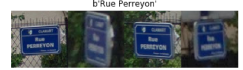
tf.data API는 메모리에 적재하기 힘든 매우 큰 데이터셋을 다룰 때, 다양한 file format을 다룰 수 있도록 도와줍니다. 예를 들어, TFRecord file format은 많은 TF app가 학습 데이터에 사용하는 간단한 record-oriented 이진 형식입니다. tf.data.TFRecordDataset 클래스는 인풋 파이프라인에서 하나 또는 그 이상의 TFRecord 파일의 내용이 흐르도록 합니다.
French Street Name Signs (FSNS)을 사용하는 예제입니다.
# Creates a dataset that reads all of the examples from two files.
fsns_test_file = tf.keras.utils.get_file("fsns.tfrec", "https://storage.googleapis.com/download.tensorflow.org/data/fsns-20160927/testdata/fsns-00000-of-00001")
TFRecordDataset을 초기화하는 filenames 인자는 string, string 배열 또는 string tf.Tensor를 전달받을 수 있습니다. 만약 학습과 검증을 위해 두 개의 파일을 사용한다면, 파일 이름을 입력으로 사용하여 데이터셋을 생성하는 팩토리 메소드로 만들 수 있습니다.
많은 데이터셋은 하나 또는 그 이상의 text 파일에 분산되어 있습니다. tf.data.TextLineDataset은 준비된 텍스트 파일에서 line 단위로 추출하는 쉬운 방법을 제공합니다. 주어진 하나 또는 그 이상의 파일 이름에서, TExtLineDataset은 line 단위로 string-value를 생성해 줄 것입니다.
directory_url = 'https://storage.googleapis.com/download.tensorflow.org/data/illiad/'
file_names = ['cowper.txt', 'derby.txt', 'butler.txt']

file_paths = [
    tf.keras.utils.get_file(file_name, directory_url + file_name)
    for file_name in file_names
]
dataset = tf.data.TextLineDataset(file_paths)
첫 번째 파일의 5개 행을 보여줍니다.
for line in dataset.take(5):
  print(line.numpy())
b"\xef\xbb\xbfAchilles sing, O Goddess! Peleus' son;" b'His wrath pernicious, who ten thousand woes' b"Caused to Achaia's host, sent many a soul" b'Illustrious into Ades premature,' b'And Heroes gave (so stood the will of Jove)'
Dataset.interleave는 파일을 번갈아 가면서 사용할 수 있게 해줍니다. 다음은 각 파일에서 나오는 문장의 예를 보여줍니다. cycle_length=3이므로 파일당 3개의 행씩 번갈아가면서 보여주겠군요.
files_ds = tf.data.Dataset.from_tensor_slices(file_paths)
lines_ds = files_ds.interleave(tf.data.TextLineDataset, cycle_length=3)

for i, line in enumerate(lines_ds.take(9)):
  if i % 3 == 0:
    print()
  print(line.numpy())
b"\xef\xbb\xbfAchilles sing, O Goddess! Peleus' son;" b"\xef\xbb\xbfOf Peleus' son, Achilles, sing, O Muse," b'\xef\xbb\xbfSing, O goddess, the anger of Achilles son of Peleus, that brought'
b'His wrath pernicious, who ten thousand woes' b'The vengeance, deep and deadly; whence to Greece' b'countless ills upon the Achaeans. Many a brave soul did it send'
b"Caused to Achaia's host, sent many a soul" b'Unnumbered ills arose; which many a soul' b'hurrying down to Hades, and many a hero did it yield a prey to dogs and'
기본적으로 TextLineDataset은 파일의 모든 line을 살펴보기 때문에 만약 파일에 header 행이나 주석이 포함된 경우 사용이 바람직하지 않을 수 있습니다. header 행이나 주석과 같은 불필요한 내용은 Dataset.skip(), Dataset.filter()를 사용하여 배제할 수 있습니다. 다음 예제는 첫 번째 행을 건너뛰고, 생존자 데이터만 찾는 경우입니다.
만약 메모리에 데이터가 존재한다면 Dataset.from_tensor_slices를 사용하여 사전 형태로 쉽게 불러올 수 있습니다.
titanic_slices = tf.data.Dataset.from_tensor_slices(dict(df))

for feature_batch in titanic_slices.take(1):
  for key, value in feature_batch.items():
    print("  {!r:20s}: {}".format(key, value))
take(1)을 통해 1 크기의 배치를 불러오고, dict 형태이기 때문에 items()로 value, key를 받습니다.
for feature_batch, label_batch in titanic_batches.take(1):
  print("'survived': {}".format(label_batch))
  print("features:")
  for key, value in feature_batch.items():
    print("  {!r:20s}: {}".format(key, value))
for feature_batch, label_batch in titanic_batches.take(1):
  print("'survived': {}".format(label_batch))
  for key, value in feature_batch.items():
    print("  {!r:20s}: {}".format(key, value))
# Creates a dataset that reads all of the records from two CSV files, each with
# four float columns which may have missing values.

record_defaults = [999,999,999,999]
dataset = tf.data.experimental.CsvDataset("missing.csv", record_defaults)
dataset = dataset.map(lambda *items: tf.stack(items))
dataset
기본적으로 CsvDataset은 모든 행과 열을 반환합니다. 이는 header 행 또는 원하는 column이 포함되어 있는 경우 바람직하지 않을 수 있습니다. header와 select_cols 인자를 통해 제거할 수 있습니다.
# Creates a dataset that reads all of the records from two CSV files with
# headers, extracting float data from columns 2 and 4.
record_defaults = [999, 999] # Only provide defaults for the selected columns
dataset = tf.data.experimental.CsvDataset("missing.csv", record_defaults, select_cols=[1, 3])
dataset = dataset.map(lambda *items: tf.stack(items))
dataset