대학원생이 쉽게 설명해보기

ABSTRACT

This paper introduces WaveNet, a deep neural network for generating raw audio waveforms. The model is fully probabilistic and autoregressive, with the predictive distribution for each audio sample conditioned on all previous ones; nonetheless we show that it can be efficiently trained on data with tens of thousands of samples per second of audio. When applied to text-to-speech, it yields state-of-the-art performance, with human listeners rating it as significantly more natural sounding than the best parametric and concatenative systems for both English and Mandarin. A single WaveNet can capture the characteristics of many different speakers with equal fidelity, and can switch between them by conditioning on the speaker identity. When trained to model music, we find that it generates novel and often highly realistic musical fragments. We also show that it can be employed as a discriminative model, returning promising results for phoneme recognition.

이 논문은 audio waveforms를 생성하기 위한 WaveNet을 소개한다.

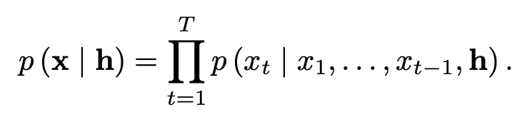
이 모델은 완전히 확률적이고 오토리그레시브하며, 각 오디오 샘플에 대한 예측 분포를 이전 모든 샘플에 맞춰 조정한다; 그럼에도 불구하고 우리는 초당 수만개의 오디오 샘플을 사용하여 효율적으로 학습이 가능하다는 것을 보여준다. 

TTS (text-to-speech)에 적용하면 최첨단 성능을 얻을 수 있으며, 청취자는 영어와 만다린 모두를 위한 최고의 파라메트릭 및 연결 시스템보다 훨씬 더 자연스러운 소리로 평가한다.

단일 WaveNet은 동일한 충실도로 서로 다른 말하는 사람들의 특징을 잡아낼 수 있고, 그들의 본질(남자 목소리, 여자 목소리 등등)을 전환하여 사용할 수 있다.

음악을 학습했을 때,  새롭고 현실적인 음악적 요소를 잘 생성한다는 것을 볼 수 있었다.

또한, 음소 인식에 대해 좋은 결과를 보여주는 적대적 모델로서 사용할 수 있다.

요약

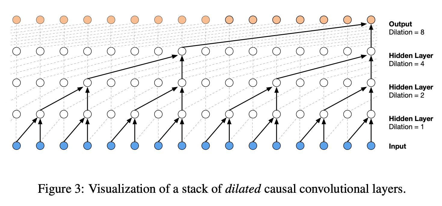
• 이 논문은 확률의 marginalization과 같이 이를 스태킹한 컨볼루션 형태로 표현하겠다는 것이 핵심이다.(Stack of Causal Convolutional Layers)

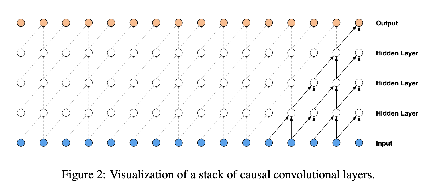
• 위의 그림을 보면, 이전의 샘플을 컨볼루션에 사용하는 것을 볼 수 있다. 예를 들어, input에서 hidden layer로 넘어갈 때 hidden layer는 각각 2개의 파란색 점을 사용함.
• 하지만 위의 그림에서의 방법은 receptive field가 작기때문에 dilated 방법을 사용한다.

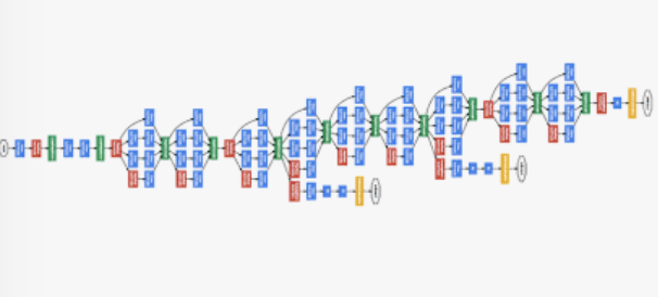
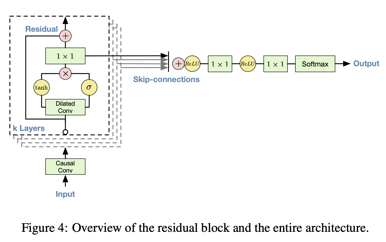
• 아키텍쳐는 다음과 같다.

• 마지막으로 Conditional WaveNet은 아래 그림과 같이 h에 어떠한 조건을 걸겠다는 것을 의미한다.

• 두 가지가 있는데, 먼저 Global Conditioning은 목소리와 같은 경우 남자 목소리는 시간이 지나도 남자 목소리이므로, 전체 타임스텝에 같은 조건을 다루도록 한다.

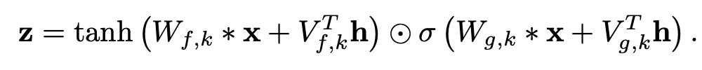
• Local Conditioning은 Condition이 시간에 따라 변하는 것이다. 이는 매우 천천히 변하는 데이터(ex: 텍스트 데이터, 텍스트 데이터는 음성 데이터에 비해 변화가 더 적음)에 적용하기 위해 transposed CNN을 사용하여 크기를 맞춰주고 1x1 CNN으로 더해주게 된다.(밑의 그림에서 V * y에서 y 부분)

Reference

Oord, A. V. D., Dieleman, S., Zen, H., Simonyan, K., Vinyals, O., Graves, A., ... & Kavukcuoglu, K. (2016). Wavenet: A generative model for raw audio. arXiv preprint arXiv:1609.03499.

ABSTRACT

Despite recent advances, memory-augmented deep neural networks are still limited when it comes to life-long and one-shot learning, especially in remembering rare events. We present a large-scale life-long memory module for use in deep learning. The module exploits fast nearest-neighbor algorithms for efficiency and thus scales to large memory sizes. Except for the nearest-neighbor query, the module is fully differentiable and trained end-to-end with no extra supervision. It operates in a life-long manner, i.e., without the need to reset it during training.

Our memory module can be easily added to any part of a supervised neural network. To show its versatility we add it to a number of networks, from simple convolutional ones tested on image classification to deep sequence-to-sequence and recurrent-convolutional models. In all cases, the enhanced network gains the ability to remember and do life-long one-shot learning. Our module remembers training examples shown many thousands of steps in the past and it can successfully generalize from them. We set new state-of-the-art for one-shot learning on the Omniglot dataset and demonstrate, for the first time, life-long one-shot learning in recurrent neural networks on a large-scale machine translation task.

최근 기술 발전에도 불구하고, 깊은 신경망의 one-shot learning과 liefe-long learning에서는 여전히 희귀 이벤트에 대해서 제한적이다. 

우리는 이를 딥러닝에서도 원활하게 사용할 수 있도록 하는 large-scale life-long memory module을 소개한다.

이 모듈은 효율성을 위한 빠른 최근접 이웃 알고리즘을 사용하여 큰 메모리 크기로 확장한다.

최근접 이웃 쿼리를 제외하고, 모듈은 완전히 미분가능하며 어떠한 감독 없이 엔드-투-엔드 방식으로 학습할 수 있다.

life-long의 관점에서 작동하며, 학습하는 동안 재설정이 필요하지 않다.

우리가 제안한 메모리 모듈은 지도학습에 쉽게 추가될 수 있다. 

모듈의 다양성을 확인해보기 위해 이미지 분류에서 간단한 컨볼루션, 심층 시퀀스-시퀀스, 순환-컨볼루션 모델에 추가해본다.

모든 경우에서 life-long one-shot learning을 실현할 수 있었다.

이 모듈은 과거의 수천 단계에서 보았던 훈련 샘플을 기억하고, 이를 성공적으로 일반화할 수 있다. 

우리는 Omniglot 데이터셋에서 이를 사용해보았고, 대규모 기계 번역 작업에서 순환신경망을 사용하여 이를 최초로 사용해보았다.

요약

• 먼저 rare events란, 어떤 데이터셋에서 매우 희귀하게 나타나는 데이터를 의미한다. 
• 기존의 신경망은 이러한 rare evenets를 기억하기에는 그래디언트 기반에서 매우 학습이 느리기 때문에 잘 반영되지 않는 문제점이 있다. 따라서 이 논문의 핵심은 신경망에 메모리 모듈을 합친다는 것이다.

• 메모리 모듈은 Key(신경망의 활성화 층 값), Value(Ground Truth의 레이블), Age(실제 이 아이템이 어느정도 저장되어 있는지 추적될 수 있도록 하는 값)으로 이루어져 있다. 
•  메모리를 사용하기 위해 쿼리를 날리는데, 여기서 쿼리는 key-size만큼의 벡터를 의마한다.
• 메모리 모듈의 학습과 업데이트는 맞은 경우, 틀린 경우로 나뉘어진다. 맞은 경우는 키값과 쿼리를 합쳐서 새로 업데이트를 하고, 틀린 경우는 여유 공간을 찾아서 그곳의 K, V, A를 다시 계산한다.
• 이 모듈은 어려운 문자로 구성되어 있는 omniglot 데이터셋과 번역에서 좋은 성능을 보여주었으며, 여러 레이어에 연결하여 편리하게 사용할 수 있다.

Reference

Kaiser, Ł., Nachum, O., Roy, A., & Bengio, S. (2017). Learning to remember rare events. arXiv preprint arXiv:1703.03129.

Abstract

How can we explain the predictions of a black-box model? In this paper, we use influence functions — a classic technique from robust statistics — to trace a model’s prediction through the learning algorithm and back to its training data, thereby identifying training points most responsible for a given prediction. To scale up influence functions to modern machine learning settings, we develop a simple, efficient implementation that requires only oracle access to gradients and Hessian-vector products. We show that even on non-convex and non-differentiable models where the theory breaks down, approximations to influence functions can still provide valuable information. On linear models and convolutional neural networks, we demonstrate that influence functions are useful for multiple purposes: understanding model behavior, debugging models, detecting dataset errors, and even creating visually-indistinguishable training-set attacks.

블랙박스 모델의 예측을 어떻게 설명할까요?

본 논문에서는 고전적인 통계 기법을 사용하여 학습 알고리즘을 통해 얻어진 모델의 예측을 영향 함수를 사용하여 추적해보고, 주어진 예측을 주는 모델이 또다른 학습 데이터를 받았을 때 어떤 영향을 보이는지 알아본다.(즉 훈련 데이터에서 해당 데이터를 없앴을 때, 예측에 어떤 영향을 끼치는가?)

현대 머신러닝을 위한 영향함수의 확장을 위해서, 간단히 Hessian-vector 내적과 그래디언트를 요구하는 방법을 개발하였다.

학습에 부정적 영향을 끼치는 non-convex나 non-differentialble의 특성을 가지고 있는 모델이 여전히 가치있는 정보를 제공할 수 있음을 영향 함수를 통해 확인하였다.

선형 모델이나 컨볼루션 신경망에서 영향 함수가 다양한 목적에 있어 유용하다는 점을 증명하였다: 모델의 행동 이해, 모델 디버깅, 데이터셋 에러 감지, 시각적으로 구분 불가능한 훈련 세트의 에러.

요약

• 이 논문은 모델이 에측할 때, 대체 왜 그런 예측을 만들었는지에 대한 질문의 답변을 생각해본 논문이다.
• 이 논문은 영향 함수를 사용하여 각 모델이 어떤 훈련 데이터에서 가장 영향을 받는지에 대한 예시를 밑의 그림에서 볼 수 있다. SVM은 픽셀단위에 예민함을 보이며, 예시 사진을 보면 주황색이 많이 들어간 사진들이 해당한다.(두 번째 행, 단순 주황색) 하지만 본 논문에서 사용된 Inception, 신경망의 경우는 표현을 학습하기 때문에 좀 더 복잡한 사진이 영향을 끼치는 것을 볼 수 있다.(세 번째 행, 주황색, 물고기 등) 

• 논문에서는 모델 파라미터에 대한 영향력, loss에 대한 영향력, input space의 변화에 대한 영향력에 대해 설명한다.

• 위의 예는 로지스틱 회귀에서 7과 1을 구분하는 문제이다. 초록색은 Training과 test가 7, 빨강색은 Training 1, test 7인 것을 의미한다. (a)는 각각 위의 식에서 train loss, Hessian, train_loss + Hessian을 빼본 것의 결과이다. (b)와 같은 경우는 테스트 이미지가 7일 때, 오른쪽 이미지를 7이라고 훈련시킨 경우에는 왼쪽 이미지를 예측하기가 힘들어진다는 것을 의미한다.  
• Loss가 non-convex이면, quadratic loss로 가정하고 했더니 잘된다. 

• Loss가 미분 불가능하면, 근사를 해서 미분 가능한 함수로 바꾸면 된다. 이 경우에는 대충 근사해도 잘되는 걸 확인할 수 있었다.

• 영향 함수는 각각의 훈련 데이터에 대한 영향을 알아볼 수 있으며, 도메인 미스매치를 디버깅할 수 있다. 또한, mislabel 문제에 대해서도 잡아낼 수 있는 장점이 있다.

Reference

Koh, P. W., & Liang, P. (2017, August). Understanding black-box predictions via influence functions. In Proceedings of the 34th International Conference on Machine Learning-Volume 70 (pp. 1885-1894). JMLR. org.

이번 글은 PR12의 유재준님께서 Inception과 Xception을 동시에 다루는 관계로 Abstract는 생략하고 바로 요약단계로 넘어가는 것으로 하겠습니다. PR12는 현재 Season 3까지 만들어져, 현재 진행중인 스터디입니다. 블로그에 게시되는 논문은 주로 Season 1에서 다루는 것들을 공부합니다. 이 글이 부족하다면 다음 유재준님께서 발표하신 영상을 보시면 되겠습니다. 

링크로는 유튜브 대신 유재준님의 블로그를 올려두겠습니다. 

http://jaejunyoo.blogspot.com/2018/02/pr12-video-34-inception-and-xception.html

요약

• Inception을 처음 고안한 모델은 GoogLeNet이다. 모델 구조는 다음과 같다.

• Xception은 성능 향상을 위해 극단적인 방법을 사용한 구조이다. 

• 먼저 Inception V1은 이미지 분류와 같은 문제를 풀기 위해 더욱 깊게 층을 쌓으려고 한 모델이다. 하지만 깊이 쌓을수록 파라미터의 수가 늘어나고, 컴퓨터 자원적으로도 매우 한계가 있게 된다. 
• 이 다음으로 층을 깊게 쌓는 것에 대한 수학적 증명 같은 것을 설명해 주시는데, 결론은 sparse connection을 이용하여 계산을 진행할 경우 수학적으로 좋다고 증명이 되었지만 컴퓨터 자원적으로 단점이 존재한다. 반면, dense connection은 수학적으로 좋지 않다고 증명이 되어있지만, 컴퓨터 자원적으로 효율적이다. 
• 기존 Inception 모듈은 1x1 컨볼루션을 사용하지 않은 구조였는데, 이는 파라미터가 급격히 증가되기 때문에 잘 작동하지 않았다. 이를 이유로 1x1 컨볼루션을 파라미터를 효율적으로 줄이고, 표현력을 풍부하게 하도록 하였다.
• Inception V2는 5x5 -> 3x3 + 3x3으로 변경하여 사용하였고, 이를 통해 28%의 파라미터 감소 효과를 누렸다.

•  이후 Xception 논문에서는 Inception 모듈이 왜 잘되는지에 대해 분석해놓았는데, 첫 번쨰로는 1x1 컨볼루션과 다양한 크기의 컨볼루션을 사용하여 채널별 상관관계와 공간적 상관관계를 동시에 적절히 수행하였다는 점이다. 
• Xception은 inception 모듈을 'extreme'하게 표현한 것인데, 여기서 Depthwise separable convolution이라는 용어가 나오게 된다.
• Depthwise separable convolution은 기존의 1x1 -> 3x3의 순서를 3x3 -> 1x1로 변경한 것이다. 이를 다시 말하면 먼저 channel-wise의 연산을 수행한 뒤, point-wise의 연산을 수행한다는 것이다.
• Inception 모듈은 기존 컨볼루션 방식과 Xception 논문에서 나오는 Depthwise separable convolution의 중간 어딘가쯤 존재하는 것이었다. 즉, Xception은 채널, 공간적 관계를 완전히 쪼개서 수행해보겠다는 것이 가설이다. 

1x1 Convolution은 Network in network 논문에서 주로 다룬 개념입니다. 

Lin, M., Chen, Q., & Yan, S. (2013). Network in network. arXiv preprint arXiv:1312.4400.

이 글에서는 MNIST 데이터셋을 Dense 층(fully-connected layer)를 사용하지 않고 학습하는 방법을 다루겠습니다.

코딩 방법에 따라 2가지로 나뉘어서 모델을 구성할 수 있습니다. 직접 돌려보니 정확도는 약 98%정도 나왔습니다.

1. 단순하게 Global Avaerage Pooling만 사용

import tensorflow as tf

(x_train, y_train), (x_test, y_test) = tf.keras.datasets.mnist.load_data()

x_train = x_train.reshape(-1,28, 28, 1)
x_train = x_train / 255
x_test = x_test.reshape(-1, 28, 28, 1)
x_test = x_test / 255

from tensorflow.keras.layers import Input, Conv2D, GlobalAveragePooling2D, MaxPooling2D
from tensorflow.keras.models import Model


inputs = Input(shape = (28, 28, 1))
x = Conv2D(32, (3, 3), strides = (1, 1), padding = 'same', activation = 'relu')(inputs)
x = MaxPooling2D(strides = (2, 2))(x)
x = Conv2D(64, (3, 3), strides = (1, 1), padding = 'same', activation = 'relu')(x)
x = MaxPooling2D(strides = (2, 2))(x)
x = Conv2D(64, (3, 3), strides = (1, 1), padding = 'same', activation = 'relu')(x)
x = MaxPooling2D(strides = (2, 2))(x)
x = Conv2D(10, (1, 1), activation = 'softmax')(x)
x = GlobalAveragePooling2D()(x)

model = Model(inputs = inputs, outputs = x)

model.compile(optimizer = 'adam', 
              loss = 'sparse_categorical_crossentropy', 
              metrics = ['acc'])
model.fit(x_train, y_train, 
          epochs = 10, batch_size = 32)

2. 적절한 Reshape 혼합

import tensorflow as tf

(x_train, y_train), (x_test, y_test) = tf.keras.datasets.mnist.load_data()

x_train = x_train.reshape(-1,28, 28, 1)
x_train = x_train / 255
x_test = x_test.reshape(-1, 28, 28, 1)
x_test = x_test / 255

from tensorflow.keras.layers import Input, Conv2D, Reshape
from tensorflow.keras.layers import GlobalAveragePooling2D, MaxPooling2D
from tensorflow.keras.models import Model


inputs = Input(shape = (28, 28, 1))
x = Conv2D(32, (3, 3), strides = (1, 1), padding = 'same', activation = 'relu')(inputs)
x = MaxPooling2D(strides = (2, 2))(x)
x = Conv2D(64, (3, 3), strides = (1, 1), padding = 'same', activation = 'relu')(x)
x = MaxPooling2D(strides = (2, 2))(x)
x = Conv2D(64, (3, 3), strides = (1, 1), padding = 'same', activation = 'relu')(x)
x = MaxPooling2D(strides = (2, 2))(x)
x = Conv2D(128, (1, 1), padding = 'same', activation = 'relu')(x)
x = GlobalAveragePooling2D()(x)
x = Reshape((1, 1, 128))(x)
x = Conv2D(10, (1, 1), padding = 'same', activation = 'softmax')(x)
x = Reshape((10,))(x)

model = Model(inputs = inputs, outputs = x)

model.compile(optimizer = 'adam', 
              loss = 'sparse_categorical_crossentropy', 
              metrics = ['acc'])
model.fit(x_train, y_train, 
          epochs = 10, batch_size = 32)

위에서 소개한 2가지 방법의 차이는 거의 없습니다. 이렇게도 할 수 있구나...를 보여주기 위해서

1x1 conv에 익숙하지 않은 분들에게 도움이 되길 바랍니다.