In this paper we describe a new mobile architecture, MobileNetV2, that improves the state of the art perfor- mance of mobile models on multiple tasks and bench- marks as well as across a spectrum of different model sizes. We also describe efficient ways of applying these mobile models to object detection in a novel framework we call SSDLite. Additionally, we demonstrate how to build mobile semantic segmentation models through a reduced form of DeepLabv3 which we call Mobile DeepLabv3.
is based on an inverted residual structure where the shortcut connections are between the thin bottle- neck layers. The intermediate expansion layer uses lightweight depthwise convolutions to filter features as a source of non-linearity. Additionally, we find that it is important to remove non-linearities in the narrow layers in order to maintain representational power. We demon- strate that this improves performance and provide an in- tuition that led to this design.
Finally, our approach allows decoupling of the in- put/output domains from the expressiveness of the trans- formation, which provides a convenient framework for further analysis. We measure our performance on ImageNet [1] classification, COCO object detection [2], VOC image segmentation [3]. We evaluate the trade-offs between accuracy, and number of operations measured by multiply-adds (MAdd), as well as actual latency, and the number of parameters.
본 논문에서는 다양한 모델 크기의 스펙트럼에서뿐만 아니라 여러 작업과 벤치마크에서 SOTA를 달성한 MobileNetV2를 소개한다.
우리는 또한 SSDLite라 부르는 새로운 프레임워크에서 이러한 모바일 모델을 객체 인식에 적용할 수 있는 효과적인 방법을 설명한다.
더하여서, 우리는 Mobile DeepLabv3이라고 부르는 축소된 DeepLabv3를 통해 어떻게 모바일 semantic segmentation을 빌드하는지 설명한다.
DeepLabv3는 shortcut connection이 병목 레이어 사이에 있는 inverted 잔차 연결 구조를 기반으로 한다.
중간 팽창 레이어는 lightweight depthwise convolutoin을 사용하여 비선형성으로서 feature들을 필터링한다.
또한, 우리는 표현력을 유지하기 위해서는 좁은 층에서 비선형성을 제거하는 것이 중요하다는 것을 알게 된다.
우리는 이것이 성능을 향상시키고 이러한 디자인을 이끌어낸 직관력을 제공한다는 것을 증명한다.
마지막으로, 우리의 방법은 추가 분석을 위한 편리한 프레임워크를 제공하는 변환의 표현성으로부터 input/output 도메인의 분리를 가능케 한다.
우리는 Imagenet 분류, COCO 객체인식, VOC 이미지 segmentation에서 실험하였다.
우리는 정확도와 multiply-adds(MAdd)를 이용하여 측정한 연산의 수 뿐만 아니라 실제 지연시간과 파라미터수 간의 트레이드 오프를 평가했다.
Reference
Sandler, M., Howard, A., Zhu, M., Zhmoginov, A., & Chen, L. C. (2018). Mobilenetv2: Inverted residuals and linear bottlenecks. In Proceedings of the IEEE Conference on Computer Vision and Pattern Recognition (pp. 4510-4520).
코드와 본문내용으로 짐작해보면, CustomDense를 config를 얻어 from_config를 사용하면 재사용할 수 있다~ 뭐 이런 것 같습니다.
(또, 위 2개의 예제가 name parameter에서 에러가 뜹니다. 댓글좀 달아주세요. API에 보면 name of layers인데 이름 집어넣어도 에러가 뜹니다) -> 그래프 초기화가 안되서 그런것 같습니다, 그냥 input_shape[-1]을 4로 바꿔주시면 됩니다. 그리고 name = 'string' 아무거나 집어넣어주세요
When to use the Functional API
함수형 API를 써서 새 모델을 만들 것인지, Model의 하위클래스로서 만들것인지 어떻게 결정할까요?
일반적으로 함수형 API는 사용이 쉽고 안전하며, Model 클래스가 가지고 있지 않은 기능을 가지고 있습니다.
그러나 Model의 하위클래스로 작업을 할 경우 Tree-RNN과 같은 함수형 API로는 표현이 쉽지 않은 모델을 구축할 수 있습니다.
위의 말은 그냥 high-level과 low-level의 차이를 설명해놓은거네요. 당연하죠.
Here are the strengths of the Functional API:
함수형 API는 super(Myclass, self).__init__(...), def call(self, ...)과 같은 함수를 정의하지 않아도 됩니다.
class MLP(keras.Model):

  def __init__(self, **kwargs):
    super(MLP, self).__init__(**kwargs)
    self.dense_1 = layers.Dense(64, activation='relu')
    self.dense_2 = layers.Dense(10)

  def call(self, inputs):
    x = self.dense_1(inputs)
    return self.dense_2(x)

# Instantiate the model.
mlp = MLP()
# Necessary to create the model's state.
# The model doesn't have a state until it's called at least once.
_ = mlp(tf.zeros((1, 32)))
여러분이 위 함수를 정의하는 동안 함수형 API는 여러분의 모델을 검증할 수 있습니다.
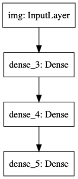
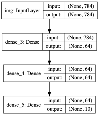
함수형 API는 plotting 및 검증이 가능합니다. - 모델을 그려볼 수도 있고, 아래와 같이 중간층도 출력하기 쉽습니다.
features_list = [layer.output for layer in vgg19.layers]
feat_extraction_model = keras.Model(inputs=vgg19.input, outputs=features_list)
Here are the weaknesses of the Functional API:
dynamic한 구조를 구축하기 어렵습니다(high-API의 단점), 전적으로 high-API의 단점을 가지고 있는거죠.
Mix-and-matching different API styles
중요한 것은, 기능 API 또는 모델 하위 분류 중 하나를 선택하는 것은 여러분을 한 범주의 모델로 제한하는 이항 결정이 아니라는 점이다. tf.keras API의 모든 모델은 시퀀셜 모델, 기능 모델 또는 처음부터 작성된 하위 분류 모델/레이어 등 각 모델과 상호 작용할 수 있다.
units = 32
timesteps = 10
input_dim = 5

# Define a Functional model
inputs = keras.Input((None, units))
x = layers.GlobalAveragePooling1D()(inputs)
outputs = layers.Dense(1, activation='sigmoid')(x)
model = keras.Model(inputs, outputs)


class CustomRNN(layers.Layer):

  def __init__(self):
    super(CustomRNN, self).__init__()
    self.units = units
    self.projection_1 = layers.Dense(units=units, activation='tanh')
    self.projection_2 = layers.Dense(units=units, activation='tanh')
    # Our previously-defined Functional model
    self.classifier = model

  def call(self, inputs):
    outputs = []
    state = tf.zeros(shape=(inputs.shape[0], self.units))
    for t in range(inputs.shape[1]):
      x = inputs[:, t, :]
      h = self.projection_1(x)
      y = h + self.projection_2(state)
      state = y
      outputs.append(y)
    features = tf.stack(outputs, axis=1)
    print(features.shape)
    return self.classifier(features)

rnn_model = CustomRNN()
_ = rnn_model(tf.zeros((1, timesteps, input_dim)))
위와 같이 함수형 API와 subclass version을 섞어서도 구성할 수 있습니다.
반대로 subclass version을 구현하여 함수형 API의 input, layer or output으로 사용할 수 있습니다. 다만, 이 방식을 사용할려면 다음과 같이 call method를 구현해야 합니다.
call(self, inputs, **kwargs)whereinputsis a tensor or a nested structure of tensors (e.g. a list of tensors), and where**kwargsare non-tensor arguments (non-inputs).
call(self, inputs, training=None, **kwargs)wheretrainingis a boolean indicating whether the layer should behave in training mode and inference mode.
call(self, inputs, mask=None, **kwargs) wheremaskis a boolean mask tensor (useful for RNNs, for instance).
call(self, inputs, training=None, mask=None, **kwargs)-- of course you can have both masking and training-specific behavior at the same time.
다음은 예시입니다.
units = 32
timesteps = 10
input_dim = 5
batch_size = 16


class CustomRNN(layers.Layer):

  def __init__(self):
    super(CustomRNN, self).__init__()
    self.units = units
    self.projection_1 = layers.Dense(units=units, activation='tanh')
    self.projection_2 = layers.Dense(units=units, activation='tanh')
    self.classifier = layers.Dense(1, activation='sigmoid')

  def call(self, inputs):
    outputs = []
    state = tf.zeros(shape=(inputs.shape[0], self.units))
    for t in range(inputs.shape[1]):
      x = inputs[:, t, :]
      h = self.projection_1(x)
      y = h + self.projection_2(state)
      state = y
      outputs.append(y)
    features = tf.stack(outputs, axis=1)
    return self.classifier(features)

# Note that we specify a static batch size for the inputs with the `batch_shape`
# arg, because the inner computation of `CustomRNN` requires a static batch size
# (when we create the `state` zeros tensor).
inputs = keras.Input(batch_shape=(batch_size, timesteps, input_dim))
x = layers.Conv1D(32, 3)(inputs)
outputs = CustomRNN()(x)

model = keras.Model(inputs, outputs)

rnn_model = CustomRNN()
_ = rnn_model(tf.zeros((1, 10, 5)))
model.save() 를 통해 모델을 저장할 수 있고, 코드가 있지 않아도 같은 구조의 모델을 load할 수 있습니다.
이 파일에는 다음과 같은 내용이 포함됨: - 모델의 아키텍처 - 모델의 weights 값(교육 중에 학습됨) - 모델의 training config(model.compile) 구성(편집하기 위해 전달된 내용), 있는 경우 - optimizer와 해당 상태(이 경우, 중단한 곳에서 교육을 다시 시작할 수 있음)
model.save('path_to_my_model.h5')
del model
# Recreate the exact same model purely from the file:
model = keras.models.load_model('path_to_my_model.h5')
Using the same graph of layers to define multiple models
함수형 API는 구체적으로 입출력을 지정할 수 있습니다. 이는 다중 입출력 모델 또한 구성 가능하다는 것을 뜻합니다.
아래 예시는 2 Model로 auto-encoder를 구성하는 것을 나타냅니다.
encoder_input = keras.Input(shape=(28, 28, 1), name='img')
x = layers.Conv2D(16, 3, activation='relu')(encoder_input)
x = layers.Conv2D(32, 3, activation='relu')(x)
x = layers.MaxPooling2D(3)(x)
x = layers.Conv2D(32, 3, activation='relu')(x)
x = layers.Conv2D(16, 3, activation='relu')(x)
encoder_output = layers.GlobalMaxPooling2D()(x)
encoder = keras.Model(encoder_input, encoder_output, name='encoder')
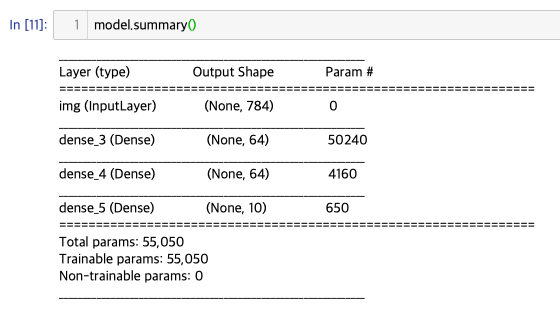
encoder.summary()
x = layers.Reshape((4, 4, 1))(encoder_output)
x = layers.Conv2DTranspose(16, 3, activation='relu')(x)
x = layers.Conv2DTranspose(32, 3, activation='relu')(x)
x = layers.UpSampling2D(3)(x)
x = layers.Conv2DTranspose(16, 3, activation='relu')(x)
decoder_output = layers.Conv2DTranspose(1, 3, activation='relu')(x)
autoencoder = keras.Model(encoder_input, decoder_output, name='autoencoder')
autoencoder.summary()
(꼭 summary()를 확인하세요!)
이러한 구성은 input_shape를 가진 output을 만들어내기 위해 필요합니다.
Conv2D의 반대는 Conv2DTranspose(가중치 학습 가능), MaxPooling2D의 받내는 UpSampling2D(가중치 학습 x)
All models are callable, just like layers
어떠한 모델이던 다른 층의 출력이나 입력을 층으로서 활용이 가능합니다. 이때, 모델 구조를 재사용하는 것이 아닌 가중치를 재사용한다는 것을 명심하세요
encoder_input = keras.Input(shape=(28, 28, 1), name='original_img')
x = layers.Conv2D(16, 3, activation='relu')(encoder_input)
x = layers.Conv2D(32, 3, activation='relu')(x)
x = layers.MaxPooling2D(3)(x)
x = layers.Conv2D(32, 3, activation='relu')(x)
x = layers.Conv2D(16, 3, activation='relu')(x)
encoder_output = layers.GlobalMaxPooling2D()(x)

encoder = keras.Model(encoder_input, encoder_output, name='encoder')
encoder.summary()

decoder_input = keras.Input(shape=(16,), name='encoded_img')
x = layers.Reshape((4, 4, 1))(decoder_input)
x = layers.Conv2DTranspose(16, 3, activation='relu')(x)
x = layers.Conv2DTranspose(32, 3, activation='relu')(x)
x = layers.UpSampling2D(3)(x)
x = layers.Conv2DTranspose(16, 3, activation='relu')(x)
decoder_output = layers.Conv2DTranspose(1, 3, activation='relu')(x)

decoder = keras.Model(decoder_input, decoder_output, name='decoder')
decoder.summary()

autoencoder_input = keras.Input(shape=(28, 28, 1), name='img')
encoded_img = encoder(autoencoder_input)
decoded_img = decoder(encoded_img)
autoencoder = keras.Model(autoencoder_input, decoded_img, name='autoencoder')
autoencoder.summary()
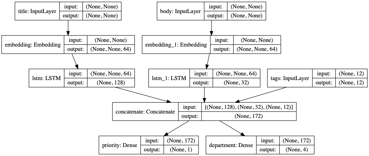
Priority score between 0 and 1 (scalar sigmoid output)
The department that should handle the ticket (softmax output over the set of departments)
코드를 볼까요.
num_tags = 12  # Number of unique issue tags
num_words = 10000  # Size of vocabulary obtained when preprocessing text data
num_departments = 4  # Number of departments for predictions

title_input = keras.Input(shape=(None,), name='title')  # Variable-length sequence of ints
body_input = keras.Input(shape=(None,), name='body')  # Variable-length sequence of ints
tags_input = keras.Input(shape=(num_tags,), name='tags')  # Binary vectors of size `num_tags`

# Embed each word in the title into a 64-dimensional vector
title_features = layers.Embedding(num_words, 64)(title_input)
# Embed each word in the text into a 64-dimensional vector
body_features = layers.Embedding(num_words, 64)(body_input)

# Reduce sequence of embedded words in the title into a single 128-dimensional vector
title_features = layers.LSTM(128)(title_features)
# Reduce sequence of embedded words in the body into a single 32-dimensional vector
body_features = layers.LSTM(32)(body_features)

# Merge all available features into a single large vector via concatenation
x = layers.concatenate([title_features, body_features, tags_input])

# Stick a logistic regression for priority prediction on top of the features
priority_pred = layers.Dense(1, activation='sigmoid', name='priority')(x)
# Stick a department classifier on top of the features
department_pred = layers.Dense(num_departments, activation='softmax', name='department')(x)

# Instantiate an end-to-end model predicting both priority and department
model = keras.Model(inputs=[title_input, body_input, tags_input],
                    outputs=[priority_pred, department_pred])
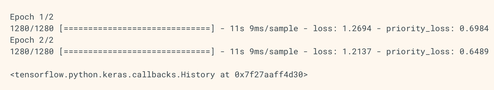
loss 또한, 각각 output에 대해 적절한 함수를 적용할 수 있습니다.
추가로 가중치를 줘서 각각 loss값이 total loss에 미치는 영향도를 조절할 수도 있습니다.
밑의 예시는 한가지 임베딩 층에 두가지 입력을 넣어 재사용성을 높였고, 여러 입력을 학습합니다.
공유 계층은 이러한 서로 다른 입력에 걸친 정보의 공유를 가능하게 하고, 그러한 모형을 더 적은 데이터로 훈련시킬 수 있게 하기 때문에 유사한 공간(예: 유사한 어휘를 특징으로 하는 두 개의 다른 텍스트)에서 오는 입력을 인코딩하는 데 자주 사용된다. 입력 중 하나에서 특정 단어가 보이는 경우, 공유 계층을 통과하는 모든 입력의 처리에 도움이 될 것이다.
# Embedding for 1000 unique words mapped to 128-dimensional vectors
shared_embedding = layers.Embedding(1000, 128)

# Variable-length sequence of integers
text_input_a = keras.Input(shape=(None,), dtype='int32')

# Variable-length sequence of integers
text_input_b = keras.Input(shape=(None,), dtype='int32')

# We reuse the same layer to encode both inputs
encoded_input_a = shared_embedding(text_input_a)
encoded_input_b = shared_embedding(text_input_b)