케라스에서 callback은 학습(epoch 시작, 끝 시점, batch의 끝시점 등)하는 동안 서로 다른 지점에서 호출되어지고, 다음과 같은 기능을 위해 사용되어집니다.
학습하는 동안 다른 지점에서 검증하기
일정 구간이나 특정 accuracy threshold를 초과할 때 모델에서 checkpointing
학습이 안정적일때 상단 레이어에서 fine-tuning
email을 보내거나 학습 종료시에 알림보내기 또는 특정 성능이 일정 수준을 초과했을 때
Etc.
Callback은 fit함수를 통해 사용할 수 있습니다.
model = get_compiled_model()

callbacks = [
    keras.callbacks.EarlyStopping(
        # Stop training when `val_loss` is no longer improving
        monitor='val_loss',
        # "no longer improving" being defined as "no better than 1e-2 less"
        min_delta=1e-2,
        # "no longer improving" being further defined as "for at least 2 epochs"
        patience=2,
        verbose=1)
]
model.fit(x_train, y_train,
          epochs=20,
          batch_size=64,
          callbacks=callbacks,
          validation_split=0.2)
Many built-in callbacks are available
ModelCheckpoint : 주기적으로 모델을 저장하기
EarlyStopping : 학습하는 동안 validation이 더이상 향상되지 않을 경우 학습을 중단하기
상대적으로 큰 데이터셋을 학습할 때, 빈번하게 모델의 체크포인트를 저장하는 것은 매우 중요합니다.
ModelCheckpoint callback을 통해 쉽게 구현할 수 있습니다.
model = get_compiled_model()

callbacks = [
    keras.callbacks.ModelCheckpoint(
        filepath='mymodel_{epoch}.h5',
        # Path where to save the model
        # The two parameters below mean that we will overwrite
        # the current checkpoint if and only if
        # the `val_loss` score has improved.
        save_best_only=True,
        monitor='val_loss',
        verbose=1)
]
model.fit(x_train, y_train,
          epochs=3,
          batch_size=64,
          callbacks=callbacks,
          validation_split=0.2)
모델을 저장하고 복원하기 위한 콜백도 직접 작성할 수 있습니다.
Using learning rate schedules
딥러닝 모델을 학습할 때 공통적인 패턴은 점진적으로 learning rate를 감소 시키는 것입니다. 이를 "learning rate decay"라고 부릅니다.
learning decay schedule은 정적(현재 epoch 또는 현재 batch index의 함수로서 미리 고정) 또는 동적(특히 검증 손실)일 수 있다.
Passing a schedule to an optimizer
우리는 optimizer에서 learning_rate인자를 통해 schedule object를 전달하면 static learning rate schedule을 쉽게 사용할 수 있습니다.
내장된 함수는 다음과 같습니다 : ExponentialDecay, PiecewiseConstantDecay, PolynomialDecay and InverseTimeDecay
Using callbacks to implement a dynamic leraning rate schedule
동적 learning rate schedule(예를 들어, validation loss가 더 이상 감소하지 않을 때 lr을 감소시켜주는 경우)는 optimizer가 validation metrics에 허용되지 않는다면 이러한 스케줄을 행할 수 없습니다.
그러나 callback은 validation metrics를 포함하여 모든 평가지표에 접근할 수 있습니다! 그래서 optimizer의 현재 lr을 수정하는 callback을 사용하는 패턴을 사용할 수 있습니다. 사실, ReduceLROnPlateau callback함수로 내장되어 있습니다.
Visualizing loss and metrics during training
학습하는 동안 모델을 시각적으로 유지하는 가장 좋은 방법은 TensorBoard를 사용하는 것입니다.
학습, 평가에 대한 loss 및 metrics를 실시간으로 plot할 수 있습니다.
(optionally) layer activations에 대한 히스토그램을 시각화 할 수 있습니다.
(optionally) Embedding layers에 의해 학습된 임베딩 공간을 3D 시각화 할 수 있습니다.
pip를 통해 텐서플로우를 설치했다면 다음과 같이 사용할 수 있습니다.
tensorboard --logdir=/full_path_to_your_logs
Using the TensorBoard callback
Keras 모델로 TensorBoard를 사용할 수 있는 가장 쉬운 방법은 TensorBoard Callback함수를 사용하는 것입니다.
keras.callbacks.TensorBoard(
  log_dir='/full_path_to_your_logs',
  histogram_freq=0,  # How often to log histogram visualizations
  embeddings_freq=0,  # How often to log embedding visualizations
  update_freq='epoch')  # How often to write logs (default: once per epoch)
지금까지 loss, metrics, optimizers, validation_data, validation_split에 대해서 다루었습니다.
지금부터는 tf.data DataSet을 통해 데이터를 어떻게 다루는지 살펴보자.
tf.data API는 TensorFlow 2.0에서 빠르고 확장 가능한 방식으로 데이터를 로드하고 사전 처리하기 위한 유틸리티의 집합입니다.
DataSet을 통해 fit(), evaluate(), predict() 를 사용할 수 있습니다.
model = get_compiled_model()

# First, let's create a training Dataset instance.
# For the sake of our example, we'll use the same MNIST data as before.
train_dataset = tf.data.Dataset.from_tensor_slices((x_train, y_train))
# Shuffle and slice the dataset.
train_dataset = train_dataset.shuffle(buffer_size=1024).batch(64)

# Now we get a test dataset.
test_dataset = tf.data.Dataset.from_tensor_slices((x_test, y_test))
test_dataset = test_dataset.batch(64)

# Since the dataset already takes care of batching,
# we don't pass a `batch_size` argument.
model.fit(train_dataset, epochs=3)

# You can also evaluate or predict on a dataset.
print('\n# Evaluate')
model.evaluate(test_dataset)
DataSet은 epoch가 끝날때마다 reset되므로 다음 epoch에서 재사용되어질 수 있습니다.
이러한 DataSet으로부터 구체적인 배치의 수만큼 학습시키길 원한다면, 다음 epoch으로 넘어가기전에 DataSet을 사용하여 얼만큼의 training steps를 거칠것인지를 다루는 steps_per_epoch 인자를 사용하세요.
이렇게 하면 각 epoch때마다 DataSet이 reset되지 않고, 대신 다음 배치만큼만 사용하게됩니다. 무한하지 않은 dataset은 결국 run-out-of-data가 될 것입니다.
model = get_compiled_model()

# Prepare the training dataset
train_dataset = tf.data.Dataset.from_tensor_slices((x_train, y_train))
train_dataset = train_dataset.shuffle(buffer_size=1024).batch(64)

# Only use the 100 batches per epoch (that's 64 * 100 samples)
model.fit(train_dataset, epochs=3, steps_per_epoch=100)
Using a validation dataset
DataSet 인스턴스로 validation_data를 사용할 수 있습니다.
model = get_compiled_model()

# Prepare the training dataset
train_dataset = tf.data.Dataset.from_tensor_slices((x_train, y_train))
train_dataset = train_dataset.shuffle(buffer_size=1024).batch(64)

# Prepare the validation dataset
val_dataset = tf.data.Dataset.from_tensor_slices((x_val, y_val))
val_dataset = val_dataset.batch(64)

model.fit(train_dataset, epochs=3, validation_data=val_dataset)
각 epoch이 끝날때마다 모델은 validation loss, metrics를 계산하고, 반복할 것입니다.
validation_steps를 사용하면 steps_per_epoch과 같은 효과를 얻을 수 있습니다.
model = get_compiled_model()

# Prepare the training dataset
train_dataset = tf.data.Dataset.from_tensor_slices((x_train, y_train))
train_dataset = train_dataset.shuffle(buffer_size=1024).batch(64)

# Prepare the validation dataset
val_dataset = tf.data.Dataset.from_tensor_slices((x_val, y_val))
val_dataset = val_dataset.batch(64)

model.fit(train_dataset, epochs=3,
          # Only run validation using the first 10 batches of the dataset
          # using the `validation_steps` argument
          validation_data=val_dataset, validation_steps=10)
검증 데이터셋은 각 사용 후 재설정됩니다.(Epoch부터 Epoch까지 항상 동일한 표본에 대해 평가하게 됨).
DataSet에선 validation_split을 사용할 수 없습니다.
Other input formats supported
넘파이 배열과 DataSet외에도 Pandas dataframe, python generator를 사용해 keras를 학습시킬 수 있습니다.
일반적으로, 데이터가 작거나 메모리에 적당한 데이터라면 넘파이 배열이나 DataSets를 추천합니다.
Using sample weighting and class weighting
입력 데이터와 대상 데이터 외에도 fit() 사용 시 표본 가중치 또는 class 가중치를 모델에 전달할 수 있습니다.
Numpy data일 경우 : sample_weight, class_weight
DataSets일 경우 : (input_batch, target batch, sample_weight_batch)
"sample weights"는 총 손실을 계산할 때 각 샘플이 배치에서 얼마나 많은 가중을 받아야 하는지를 구체적으로 담은 배열입니다. 흔히 불균형 분류 문제에 사용되어집니다.(부족한 데이터를 가진 class에 더 높은 가중을 주는 경우). 사용된 가중치가 1과 0인 경우, 총 손실에 특정 샘플의 기여를 무시하는 손실 함수를 위한 mask로서 사용될 수 있습니다.
"class weights"는 클래스에 따라 샘플들이 가져야하는 가중에 대한 배열입니다. 예를 들어, 0이 1보다 2배 적다면 class_weight={0:1., 1:0.5}와 같이 사용할 수 있습니다.
다음은 클래스 가중치 또는 샘플 가중치를 사용하여 클래스 #5(MNIST 데이터 세트의 숫자 "5")의 올바른 분류에 더 중요성을 부여하는 Numpy 예입니다.
import numpy as np

class_weight = {0: 1., 1: 1., 2: 1., 3: 1., 4: 1.,
                # Set weight "2" for class "5",
                # making this class 2x more important
                5: 2.,
                6: 1., 7: 1., 8: 1., 9: 1.}
model.fit(x_train, y_train,
          class_weight=class_weight,
          batch_size=64,
          epochs=4)

# Here's the same example using `sample_weight` instead:
sample_weight = np.ones(shape=(len(y_train),))
sample_weight[y_train == 5] = 2.

model = get_compiled_model()
model.fit(x_train, y_train,
          sample_weight=sample_weight,
          batch_size=64,
          epochs=4)
다음은 DataSet을 사용한 예입니다.
sample_weight = np.ones(shape=(len(y_train),))
sample_weight[y_train == 5] = 2.

# Create a Dataset that includes sample weights
# (3rd element in the return tuple).
train_dataset = tf.data.Dataset.from_tensor_slices(
    (x_train, y_train, sample_weight))

# Shuffle and slice the dataset.
train_dataset = train_dataset.shuffle(buffer_size=1024).batch(64)

model = get_compiled_model()
model.fit(train_dataset, epochs=3)
Passing data to multi-input, multi-output models
앞의 예에서는 단일 입력(764,)와 단일 출력(10,)을 사용했습니다. 다중 입력/출력 일때는 어떻게 해야할까요?
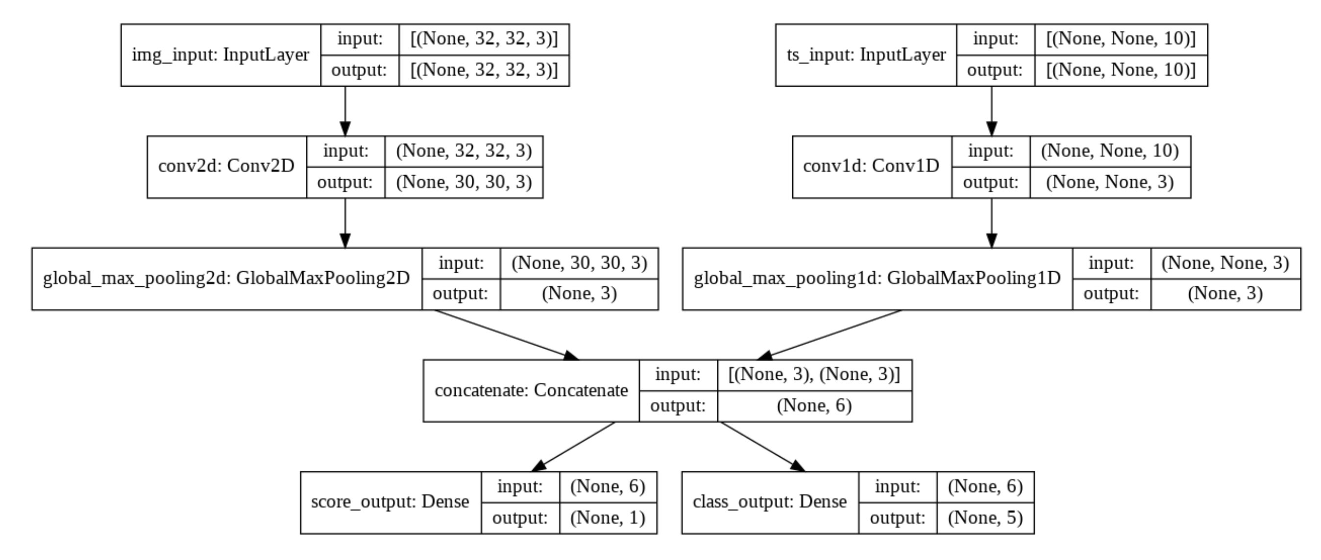
(None - timesteps, 10 - features)로 이루어진 시계열 입력과 (32, 32, 3)으로 이루어진 이미지 입력을 생각해 봅시다. 모델은 점수와 5class로 구성된 확률분포를 output으로 가집니다.
이러한 outputs이 예측이아니라 학습을 위한 것이라면, 특정 output에 대해서는 계산을 허용하지 않을 수도 있습니다.
# List loss version
model.compile(
    optimizer=keras.optimizers.RMSprop(1e-3),
    loss=[None, keras.losses.CategoricalCrossentropy()])

# Or dict loss version
model.compile(
    optimizer=keras.optimizers.RMSprop(1e-3),
    loss={'class_output': keras.losses.CategoricalCrossentropy()})
fit 함수데이터를 적합한 다중 입력 또는 다중 출력 모델로 전송하는 것은 컴파일에서 손실 함수를 지정하는 것과 유사한 방식으로 작동합니다. 넘파이 배열을 활용한 dict나 list형태를 사용할 수 있습니다.
이번 가이드는 tensorflow 2.0에서 겪을 수 있는 training, evaluation, prediction을 다룹니다.
(model.fit(), model.evaluate(), model.predict())를 사용하는 경우
eager execution and the GradientTape를 사용하는 경우
일반적으로, 여러분이 내장된 루프를 사용하든, 여러분 자신의 루프를 쓰든, 모델 훈련과 평가는 모든 종류의 케라스 모델, 즉 Sequential 모델, funtional API로 제작된 모델, 모델 하위 분류를 통해 처음부터 작성된 모델에서 엄격하게 같은 방식으로 작동한다.
이 가이드는 분산 트레이닝에 대한 내용은 다루지 않습니다.
Part 1: Using build-in training & evaluation loops
model의 내장된 traninig 루프에 데이터를 넣어줄 떄, Numpy array(데이터가 작거나 메모리에 적당한 경우)나 tf.data Dataset 객체를 사용해야만 합니다. 다음에 나오는 내용들은 optimizers, losses, metrics를 어떻게 사용하는지에 대해 numpy array를 사용한 MNIST 데이터셋에 대한 예제를 다룰 것입니다.
API overview: a first end-to-end example
다음 예제를 보자.
from tensorflow import keras
from tensorflow.keras import layers
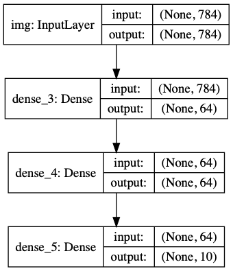
inputs = keras.Input(shape=(784,), name='digits')
x = layers.Dense(64, activation='relu', name='dense_1')(inputs)
x = layers.Dense(64, activation='relu', name='dense_2')(x)
outputs = layers.Dense(10, activation='softmax', name='predictions')(x)
model = keras.Model(inputs=inputs, outputs=outputs)
test data에 대한 평가와 train data에서 생성되는 hold out set에 대한 검증, train data로 구성되는 전형적인 end-to-end의 workflow는 다음과 같습니다.
# Load a toy dataset for the sake of this example
(x_train, y_train), (x_test, y_test) = keras.datasets.mnist.load_data()
# Preprocess the data (these are Numpy arrays)
x_train = x_train.reshape(60000, 784).astype('float32') / 255
x_test = x_test.reshape(10000, 784).astype('float32') / 255
# Reserve 10,000 samples for validation
x_val = x_train[-10000:]
y_val = y_train[-10000:]
x_train = x_train[:-10000]
y_train = y_train[:-10000]
# Specify the training configuration (optimizer, loss, metrics)
model.compile(optimizer=keras.optimizers.RMSprop(), # Optimizer
# Loss function to minimize
loss=keras.losses.SparseCategoricalCrossentropy(),
# List of metrics to monitor
metrics=[keras.metrics.SparseCategoricalAccuracy()])
# Train the model by slicing the data into "batches"
# of size "batch_size", and repeatedly iterating over
# the entire dataset for a given number of "epochs"
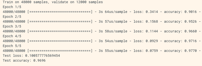
print('# Fit model on training data')
history = model.fit(x_train, y_train,
batch_size=64,
epochs=3,
# We pass some validation for
# monitoring validation loss and metrics
# at the end of each epoch
validation_data=(x_val, y_val))
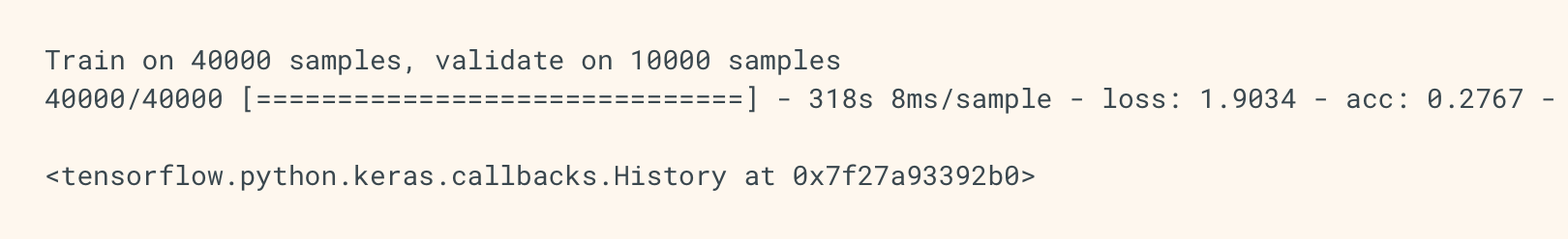
# The returned "history" object holds a record
# of the loss values and metric values during training
print('\nhistory dict:', history.history)
# Evaluate the model on the test data using `evaluate`
print('\n# Evaluate on test data')
results = model.evaluate(x_test, y_test, batch_size=128)
print('test loss, test acc:', results)
# Generate predictions (probabilities -- the output of the last layer)
# on new data using `predict`
print('\n# Generate predictions for 3 samples')
predictions = model.predict(x_test[:3])
print('predictions shape:', predictions.shape)
Specifying a loss, metrics, and an optimizer
model의 fit함수를 사용하여 train시키려면 우리는 구체적인 loss function, optimizer, metric에 대해 정의해야 합니다.
metrics 인자는 list형태여야 하며 우리가 원하는 어떠한 metric도 추가 될 수 있습니다.
만약 우리의 모델이 multiple output이라면, 각각 다른 loss와 metrics를 지정할 수 있고, total loss에 대한 영향을 조절할 수 있습니다. 향후 다룰 "Passing data to multi-input, multi-output models" section에서 더욱 자세한 내용을 찾아 볼 수 있습니다.
나중에 재사용할 수 있도록 모델 정의와 기능의 단계를 정리해 봅시다. 이 가이드의 다른 예에서 여러 번 부르기로 합시다.
def get_uncompiled_model():
inputs = keras.Input(shape=(784,), name='digits')
x = layers.Dense(64, activation='relu', name='dense_1')(inputs)
x = layers.Dense(64, activation='relu', name='dense_2')(x)
outputs = layers.Dense(10, activation='softmax', name='predictions')(x)
model = keras.Model(inputs=inputs, outputs=outputs)
return model
def get_compiled_model():
model = get_uncompiled_model()
model.compile(optimizer=keras.optimizers.RMSprop(learning_rate=1e-3),
              loss='sparse_categorical_crossentropy',
              metrics=['sparse_categorical_accuracy'])
return model
Many built-in optimizers, losses, and metrics are available
일반적으로 직접 정의하는 것 보단 Keras API에 정의된 것을 사용하는게 편할 것입니다.
Optimizers : - SGD()(with or without momentum) - RMSprop() - Adam() - etc.
Losses : - MeanSquaredError() - KLDivergence() - CosineSimilarity() - etc.
Metrics : - AUC() - Precision() - Recall() - etc.
Writing custom losses and metrics
API에 존재하지 않는 지표가 필요하다면, Metric class를 이용해 쉽게 customizing할 수 있습니다. 4개의 method가 필요합니다.
__init__(self), 우리의 metrics를 위한 state variables를 정의합니다.
update_state(self, y_true, y_pred, sample_weight=None), y_true값과 state variables를 업데이트할 y_pred를 사용합니다.
result(self), 결과를 도출합니다.
reset_states(self), 지표의 상태를 초기화합니다.
State update와 결과 도출은 결과를 계산하는 것이 매우 오래걸리기 때문에 각각 updatae_state()와 result()로 나누어져 있습니다.
아래 예제는 분류문제에서 각 Sample이 얼마나 맞췄는지에 대해 갯수를 세는 CategoricalTruePositives를 정의한 것입니다.
class CatgoricalTruePositives(keras.metrics.Metric):

    def __init__(self, name='binary_true_positives', **kwargs):
      super(CatgoricalTruePositives, self).__init__(name=name, **kwargs)
      self.true_positives = self.add_weight(name='tp', initializer='zeros')

    def update_state(self, y_true, y_pred, sample_weight=None):
      y_pred = tf.argmax(y_pred)
      values = tf.equal(tf.cast(y_true, 'int32'), tf.cast(y_pred, 'int32'))
      values = tf.cast(values, 'float32')
      if sample_weight is not None:
        sample_weight = tf.cast(sample_weight, 'float32')
        values = tf.multiply(values, sample_weight)
      return self.true_positives.assign_add(tf.reduce_sum(values))  # TODO: fix

    def result(self):
      return tf.identity(self.true_positives)  # TODO: fix

    def reset_states(self):
      # The state of the metric will be reset at the start of each epoch.
      self.true_positives.assign(0.)


model.compile(optimizer=keras.optimizers.RMSprop(learning_rate=1e-3),
              loss=keras.losses.SparseCategoricalCrossentropy(),
              metrics=[CatgoricalTruePositives()])
model.fit(x_train, y_train,
          batch_size=64,
          epochs=3)
Handling losses and metrics that don't fit the standard signature
압도적인 다수의 손실과 측정 지표는 y_true와 y_pred로 계산할 수 있습니다. 여기서 y_pred는 모델의 산출물입니다. 하지만 전부 다 그런 것은 아닙니다. 예를 들어, 정규화 손실은 계층의 활성화만 필요할 수 있으며(이 경우에는 대상이 없다), 이 활성화는 모델 출력이 아닐 수 있 수 있습니다.
이러한 경우에 우리는 custom layer의 call 메서드를 통한 self.add_loss(loss_value)를 사용할 수 있습니다.
class ActivityRegularizationLayer(layers.Layer):

  def call(self, inputs):
    self.add_loss(tf.reduce_sum(inputs) * 0.1)
    return inputs  # Pass-through layer.

inputs = keras.Input(shape=(784,), name='digits')
x = layers.Dense(64, activation='relu', name='dense_1')(inputs)

# Insert activity regularization as a layer
x = ActivityRegularizationLayer()(x)

x = layers.Dense(64, activation='relu', name='dense_2')(x)
outputs = layers.Dense(10, activation='softmax', name='predictions')(x)

model = keras.Model(inputs=inputs, outputs=outputs)
model.compile(optimizer=keras.optimizers.RMSprop(learning_rate=1e-3),
              loss='sparse_categorical_crossentropy')

# The displayed loss will be much higher than before
# due to the regularization component.
model.fit(x_train, y_train,
          batch_size=64,
          epochs=1)
metric 값 logging에 대해서도 동일한 작업을 진행할 수 있습니다.
class MetricLoggingLayer(layers.Layer):
def call(self, inputs):
# The `aggregation` argument defines
# how to aggregate the per-batch values
# over each epoch:
# in this case we simply average them.
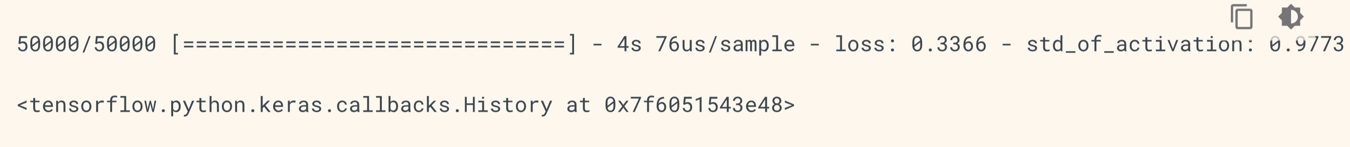
self.add_metric(keras.backend.std(inputs),
name='std_of_activation',
aggregation='mean')
return inputs # Pass-through layer.
inputs = keras.Input(shape=(784,), name='digits')
x = layers.Dense(64, activation='relu', name='dense_1')(inputs)
# Insert std logging as a layer.
x = MetricLoggingLayer()(x)
x = layers.Dense(64, activation='relu', name='dense_2')(x)
outputs = layers.Dense(10, activation='softmax', name='predictions')(x)
model = keras.Model(inputs=inputs, outputs=outputs)
model.compile(optimizer=keras.optimizers.RMSprop(learning_rate=1e-3),
loss='sparse_categorical_crossentropy')
model.fit(x_train, y_train,
batch_size=64,
epochs=1)
옆에 std_of_activation 참고
Functional API에서 또한, model.add_loss(loss_tensor) or model.add_metric(metric_tensor, name, aggregation)을 호출할 수 있습니다.
Automatically setting apart a validation holdout set
우리는 각 epoch마다 (x_val, y_val)을 통해 평가할 수 있습니다.
이를 위한 옵션이 있습니다 : validation_split 인자는 자동적으로 우리의 training_data에서 우리가 허용한 만큼 뒷 부분을 validation_data로 만듭니다. 이 인자값은 데이터에서 얼마만큼의 검증데이터를 만들 것인지를 나타내며, 0과 1사이의 값으로 조정합니다. 예를 들어, validation_split = 0.2는 traninig 데이터의 20퍼를 검증데이터로 활용하겠다는 뜻입니다.
이러한 검증 방법은 shuffling 전에 fit함수에서의 호출을 통해 데이터의 끝 x%만큼을 validation_data로 활용하게 됩니다.
model = get_compiled_model()
model.fit(x_train, y_train, batch_size=64, validation_split=0.2, epochs=3)
코드와 본문내용으로 짐작해보면, CustomDense를 config를 얻어 from_config를 사용하면 재사용할 수 있다~ 뭐 이런 것 같습니다.
(또, 위 2개의 예제가 name parameter에서 에러가 뜹니다. 댓글좀 달아주세요. API에 보면 name of layers인데 이름 집어넣어도 에러가 뜹니다) -> 그래프 초기화가 안되서 그런것 같습니다, 그냥 input_shape[-1]을 4로 바꿔주시면 됩니다. 그리고 name = 'string' 아무거나 집어넣어주세요
When to use the Functional API
함수형 API를 써서 새 모델을 만들 것인지, Model의 하위클래스로서 만들것인지 어떻게 결정할까요?
일반적으로 함수형 API는 사용이 쉽고 안전하며, Model 클래스가 가지고 있지 않은 기능을 가지고 있습니다.
그러나 Model의 하위클래스로 작업을 할 경우 Tree-RNN과 같은 함수형 API로는 표현이 쉽지 않은 모델을 구축할 수 있습니다.
위의 말은 그냥 high-level과 low-level의 차이를 설명해놓은거네요. 당연하죠.
Here are the strengths of the Functional API:
함수형 API는 super(Myclass, self).__init__(...), def call(self, ...)과 같은 함수를 정의하지 않아도 됩니다.
class MLP(keras.Model):

  def __init__(self, **kwargs):
    super(MLP, self).__init__(**kwargs)
    self.dense_1 = layers.Dense(64, activation='relu')
    self.dense_2 = layers.Dense(10)

  def call(self, inputs):
    x = self.dense_1(inputs)
    return self.dense_2(x)

# Instantiate the model.
mlp = MLP()
# Necessary to create the model's state.
# The model doesn't have a state until it's called at least once.
_ = mlp(tf.zeros((1, 32)))
여러분이 위 함수를 정의하는 동안 함수형 API는 여러분의 모델을 검증할 수 있습니다.
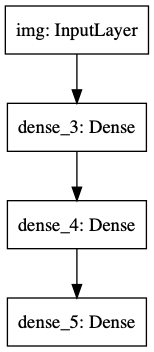
함수형 API는 plotting 및 검증이 가능합니다. - 모델을 그려볼 수도 있고, 아래와 같이 중간층도 출력하기 쉽습니다.
features_list = [layer.output for layer in vgg19.layers]
feat_extraction_model = keras.Model(inputs=vgg19.input, outputs=features_list)
Here are the weaknesses of the Functional API:
dynamic한 구조를 구축하기 어렵습니다(high-API의 단점), 전적으로 high-API의 단점을 가지고 있는거죠.
Mix-and-matching different API styles
중요한 것은, 기능 API 또는 모델 하위 분류 중 하나를 선택하는 것은 여러분을 한 범주의 모델로 제한하는 이항 결정이 아니라는 점이다. tf.keras API의 모든 모델은 시퀀셜 모델, 기능 모델 또는 처음부터 작성된 하위 분류 모델/레이어 등 각 모델과 상호 작용할 수 있다.
units = 32
timesteps = 10
input_dim = 5

# Define a Functional model
inputs = keras.Input((None, units))
x = layers.GlobalAveragePooling1D()(inputs)
outputs = layers.Dense(1, activation='sigmoid')(x)
model = keras.Model(inputs, outputs)


class CustomRNN(layers.Layer):

  def __init__(self):
    super(CustomRNN, self).__init__()
    self.units = units
    self.projection_1 = layers.Dense(units=units, activation='tanh')
    self.projection_2 = layers.Dense(units=units, activation='tanh')
    # Our previously-defined Functional model
    self.classifier = model

  def call(self, inputs):
    outputs = []
    state = tf.zeros(shape=(inputs.shape[0], self.units))
    for t in range(inputs.shape[1]):
      x = inputs[:, t, :]
      h = self.projection_1(x)
      y = h + self.projection_2(state)
      state = y
      outputs.append(y)
    features = tf.stack(outputs, axis=1)
    print(features.shape)
    return self.classifier(features)

rnn_model = CustomRNN()
_ = rnn_model(tf.zeros((1, timesteps, input_dim)))
위와 같이 함수형 API와 subclass version을 섞어서도 구성할 수 있습니다.
반대로 subclass version을 구현하여 함수형 API의 input, layer or output으로 사용할 수 있습니다. 다만, 이 방식을 사용할려면 다음과 같이 call method를 구현해야 합니다.
call(self, inputs, **kwargs)whereinputsis a tensor or a nested structure of tensors (e.g. a list of tensors), and where**kwargsare non-tensor arguments (non-inputs).
call(self, inputs, training=None, **kwargs)wheretrainingis a boolean indicating whether the layer should behave in training mode and inference mode.
call(self, inputs, mask=None, **kwargs) wheremaskis a boolean mask tensor (useful for RNNs, for instance).
call(self, inputs, training=None, mask=None, **kwargs)-- of course you can have both masking and training-specific behavior at the same time.
다음은 예시입니다.
units = 32
timesteps = 10
input_dim = 5
batch_size = 16


class CustomRNN(layers.Layer):

  def __init__(self):
    super(CustomRNN, self).__init__()
    self.units = units
    self.projection_1 = layers.Dense(units=units, activation='tanh')
    self.projection_2 = layers.Dense(units=units, activation='tanh')
    self.classifier = layers.Dense(1, activation='sigmoid')

  def call(self, inputs):
    outputs = []
    state = tf.zeros(shape=(inputs.shape[0], self.units))
    for t in range(inputs.shape[1]):
      x = inputs[:, t, :]
      h = self.projection_1(x)
      y = h + self.projection_2(state)
      state = y
      outputs.append(y)
    features = tf.stack(outputs, axis=1)
    return self.classifier(features)

# Note that we specify a static batch size for the inputs with the `batch_shape`
# arg, because the inner computation of `CustomRNN` requires a static batch size
# (when we create the `state` zeros tensor).
inputs = keras.Input(batch_shape=(batch_size, timesteps, input_dim))
x = layers.Conv1D(32, 3)(inputs)
outputs = CustomRNN()(x)

model = keras.Model(inputs, outputs)

rnn_model = CustomRNN()
_ = rnn_model(tf.zeros((1, 10, 5)))
model.save() 를 통해 모델을 저장할 수 있고, 코드가 있지 않아도 같은 구조의 모델을 load할 수 있습니다.
이 파일에는 다음과 같은 내용이 포함됨: - 모델의 아키텍처 - 모델의 weights 값(교육 중에 학습됨) - 모델의 training config(model.compile) 구성(편집하기 위해 전달된 내용), 있는 경우 - optimizer와 해당 상태(이 경우, 중단한 곳에서 교육을 다시 시작할 수 있음)
model.save('path_to_my_model.h5')
del model
# Recreate the exact same model purely from the file:
model = keras.models.load_model('path_to_my_model.h5')
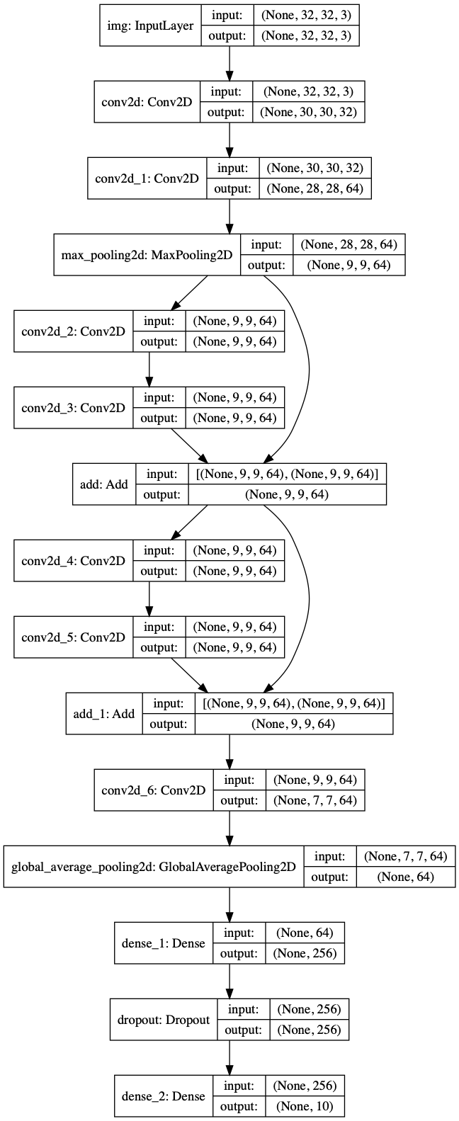
Using the same graph of layers to define multiple models
함수형 API는 구체적으로 입출력을 지정할 수 있습니다. 이는 다중 입출력 모델 또한 구성 가능하다는 것을 뜻합니다.
아래 예시는 2 Model로 auto-encoder를 구성하는 것을 나타냅니다.
encoder_input = keras.Input(shape=(28, 28, 1), name='img')
x = layers.Conv2D(16, 3, activation='relu')(encoder_input)
x = layers.Conv2D(32, 3, activation='relu')(x)
x = layers.MaxPooling2D(3)(x)
x = layers.Conv2D(32, 3, activation='relu')(x)
x = layers.Conv2D(16, 3, activation='relu')(x)
encoder_output = layers.GlobalMaxPooling2D()(x)
encoder = keras.Model(encoder_input, encoder_output, name='encoder')
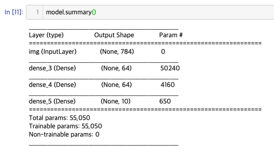
encoder.summary()
x = layers.Reshape((4, 4, 1))(encoder_output)
x = layers.Conv2DTranspose(16, 3, activation='relu')(x)
x = layers.Conv2DTranspose(32, 3, activation='relu')(x)
x = layers.UpSampling2D(3)(x)
x = layers.Conv2DTranspose(16, 3, activation='relu')(x)
decoder_output = layers.Conv2DTranspose(1, 3, activation='relu')(x)
autoencoder = keras.Model(encoder_input, decoder_output, name='autoencoder')
autoencoder.summary()
(꼭 summary()를 확인하세요!)
이러한 구성은 input_shape를 가진 output을 만들어내기 위해 필요합니다.
Conv2D의 반대는 Conv2DTranspose(가중치 학습 가능), MaxPooling2D의 받내는 UpSampling2D(가중치 학습 x)
All models are callable, just like layers
어떠한 모델이던 다른 층의 출력이나 입력을 층으로서 활용이 가능합니다. 이때, 모델 구조를 재사용하는 것이 아닌 가중치를 재사용한다는 것을 명심하세요
encoder_input = keras.Input(shape=(28, 28, 1), name='original_img')
x = layers.Conv2D(16, 3, activation='relu')(encoder_input)
x = layers.Conv2D(32, 3, activation='relu')(x)
x = layers.MaxPooling2D(3)(x)
x = layers.Conv2D(32, 3, activation='relu')(x)
x = layers.Conv2D(16, 3, activation='relu')(x)
encoder_output = layers.GlobalMaxPooling2D()(x)

encoder = keras.Model(encoder_input, encoder_output, name='encoder')
encoder.summary()

decoder_input = keras.Input(shape=(16,), name='encoded_img')
x = layers.Reshape((4, 4, 1))(decoder_input)
x = layers.Conv2DTranspose(16, 3, activation='relu')(x)
x = layers.Conv2DTranspose(32, 3, activation='relu')(x)
x = layers.UpSampling2D(3)(x)
x = layers.Conv2DTranspose(16, 3, activation='relu')(x)
decoder_output = layers.Conv2DTranspose(1, 3, activation='relu')(x)

decoder = keras.Model(decoder_input, decoder_output, name='decoder')
decoder.summary()

autoencoder_input = keras.Input(shape=(28, 28, 1), name='img')
encoded_img = encoder(autoencoder_input)
decoded_img = decoder(encoded_img)
autoencoder = keras.Model(autoencoder_input, decoded_img, name='autoencoder')
autoencoder.summary()
Priority score between 0 and 1 (scalar sigmoid output)
The department that should handle the ticket (softmax output over the set of departments)
코드를 볼까요.
num_tags = 12 # Number of unique issue tags
num_words = 10000 # Size of vocabulary obtained when preprocessing text data
num_departments = 4 # Number of departments for predictions
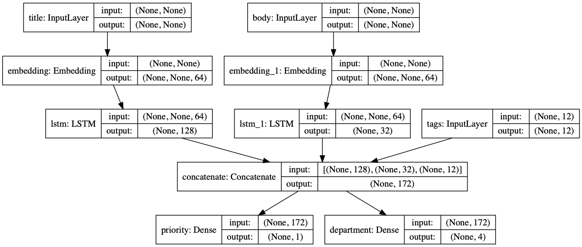
title_input = keras.Input(shape=(None,), name='title') # Variable-length sequence of ints
body_input = keras.Input(shape=(None,), name='body') # Variable-length sequence of ints
tags_input = keras.Input(shape=(num_tags,), name='tags') # Binary vectors of size `num_tags`
# Embed each word in the title into a 64-dimensional vector
title_features = layers.Embedding(num_words, 64)(title_input)
# Embed each word in the text into a 64-dimensional vector
body_features = layers.Embedding(num_words, 64)(body_input)
# Reduce sequence of embedded words in the title into a single 128-dimensional vector
title_features = layers.LSTM(128)(title_features)
# Reduce sequence of embedded words in the body into a single 32-dimensional vector
body_features = layers.LSTM(32)(body_features)
# Merge all available features into a single large vector via concatenation
x = layers.concatenate([title_features, body_features, tags_input])
# Stick a logistic regression for priority prediction on top of the features
priority_pred = layers.Dense(1, activation='sigmoid', name='priority')(x)
# Stick a department classifier on top of the features
department_pred = layers.Dense(num_departments, activation='softmax', name='department')(x)
# Instantiate an end-to-end model predicting both priority and department
model = keras.Model(inputs=[title_input, body_input, tags_input],
outputs=[priority_pred, department_pred])
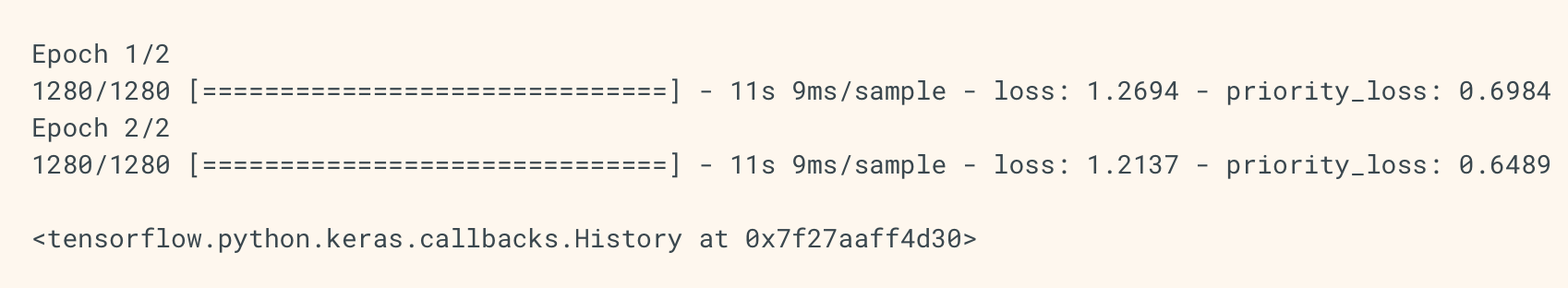
loss 또한, 각각 output에 대해 적절한 함수를 적용할 수 있습니다.
추가로 가중치를 줘서 각각 loss값이 total loss에 미치는 영향도를 조절할 수도 있습니다.
밑의 예시는 한가지 임베딩 층에 두가지 입력을 넣어 재사용성을 높였고, 여러 입력을 학습합니다.
공유 계층은 이러한 서로 다른 입력에 걸친 정보의 공유를 가능하게 하고, 그러한 모형을 더 적은 데이터로 훈련시킬 수 있게 하기 때문에 유사한 공간(예: 유사한 어휘를 특징으로 하는 두 개의 다른 텍스트)에서 오는 입력을 인코딩하는 데 자주 사용된다. 입력 중 하나에서 특정 단어가 보이는 경우, 공유 계층을 통과하는 모든 입력의 처리에 도움이 될 것이다.
# Embedding for 1000 unique words mapped to 128-dimensional vectors
shared_embedding = layers.Embedding(1000, 128)

# Variable-length sequence of integers
text_input_a = keras.Input(shape=(None,), dtype='int32')

# Variable-length sequence of integers
text_input_b = keras.Input(shape=(None,), dtype='int32')

# We reuse the same layer to encode both inputs
encoded_input_a = shared_embedding(text_input_a)
encoded_input_b = shared_embedding(text_input_b)